Excel for Accountants (20 Skills to Master in 2025)

If you are an accountant, one of the most important skills for you to master is Microsoft Excel, period. Why I’m saying this? Well, financial data is what you deal with as an accountant, and you need to be good at managing and analyzing data, right?

And Microsoft Excel is the tool you need. To get started with it, you can learn:

• Introduction to Excel
• Excel Tips
• Excel Functions

BUT.

You are an accounting professional, so you also need to learn all those specific things which can help you to thrive in your work. Let me tell you that this is the most comprehensive guide you can find on the internet to help you to be a better accountant.

Below is the list of the 20 Excel Skills that every accountant needs to master this year.

1. Keyboard Shortcuts for Accountants

No matter, if you are an accountant, finance professional, or in some other profession, using keyboard shortcuts, can help you to save a lot of time.

Here’s the Excel Keyboard Shortcuts Cheat Sheet with 82 shortcuts that you can use in your daily work and below are some of them:

• Control + Shift + L Apply-Remove Filter
• Alt + = AutoSum
• Alt ⇢ H ⇢ E ⇢ A Clear Contents
• Ctrl + 1 Open Format Cells Options
• Control + 5 Strikethrough
• Alt ⇢ H ⇢ W Wrap Text
• Alt ⇢ W ⇢ F ⇢ R Freeze Top Row
• Alt + 0 ⇢ 2 ⇢ 5 ⇢ 2 Check Mark
• Shift + F2 Add Comments
• Alt ⇢ H ⇢ B ⇢ A Apply Border
• Alt + Shift + ➔ Group
• Alt ⇢ H ⇢ V ⇢ T Transpose

Here are my few tips for every accountant about keyboard shortcuts:

• Replace your 10 most used options with keyboard shortcuts.
• Try to locate shortcut keys by pressing the ALT key.

Related: Apply Accounting Number Format in Excel

2. Power of Paste Special

One of the options which you need to learn is PASTE‌ SPECIAL. With it, you can do a lot of things other than a normal paste.

To open the paste special option, you need to go to the Home Tab ➜ Clipboard ➜ Paste Special, or you can also use the shortcut key Control + Alt + V.

Once you open it you can see there are more than 16 options to use, but let me share the most useful options that you need to learn:

1. Values: It only pastes values, ignoring formulas and formatting from the source cell, and is best to use if you want to convert formulas into values.
2. Formulas: It only pastes formulas, instead of values and is best to use if you want to use apply formulas.
3. Formats: It copies and pastes the formatting, ignoring values and formulas from the source cell (Quick Tip: Format Painter).
4. Column Width: It only applies the column width to the destination column, ignoring the rest.
5. Operations: With this option, you can perform simple (multiply, divide, subtract, and add) calculations (check out this trick).

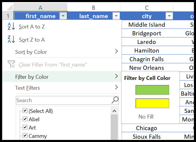
3. Sort Data Like a PRO

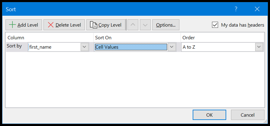
In Excel, there are multiple ways to sort data. When you open the sort dialog box (Data Tab ➜ Sort & Filter ➜ Sort), you can add a level to sort. Imagine if you want to sort the below data using the first_name column, you need to add a sorting level for this:

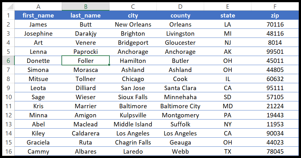
1. First of all, select the column from the “Sort By”.
2. After that, in “Sort On”, select “Cell Values”.
3. In the end, in “Order”, A to Z.

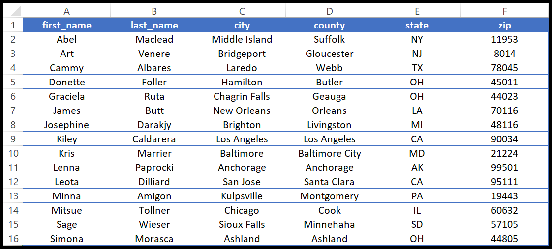
Once you click OK, you’ll get the data sorted like below:

Well, this was the basic way to sort data which is mostly used, but apart from that, there are some advanced sorting options that you can use.

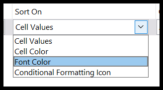
1. Sort On

From the “Sort On” drop-down, you can select the option to sort with font color, cell color, or conditional formatting.

So if you select the cell color, it gives you the further option to show it on the top or at the bottom after sorting.

2. Custom List

You can also create a custom list of sorting values. Imagine you have a list of names and you want all the names in a particular order, you can create a custom list for that.

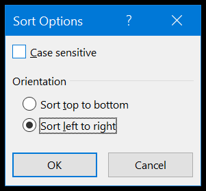
3. Sorting Column

By default, when you use the sort option it sort by rows but there’s an option that helps you to sort data by column. Open the “Options” and tick mark “Sort Left to Right”.

Related: Sort By Date, Date and Time & Reverse Date Sort

4. Advanced Options to Filter Data

Excel filter is fast and powerful. It gives different ways to filter data from a column. When you open a filter you can see there are a lot of options that you can use.

Below I have listed the most useful options which you can use:

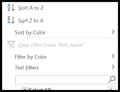
1. Filter by Color

So if you have cell color, font color, or even applied conditional formatting, you can filter all those cells as well.

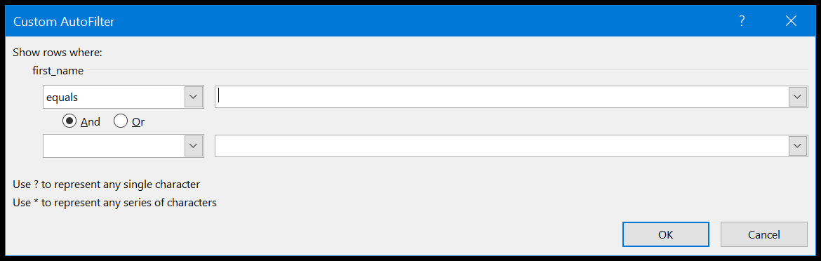
2. Custom Filter

With a custom filter, you can filter using conditions, partial matches, wildcard characters, and much more.

3. Date Filters

If you have dates in the column, you can use date filters to filter them in different ways, like weeks, months, and years.

4. Search Box

With the search box, you can filter values in a flash. You just need to type the value and hit enter.

Quick Tip: You can also filter values by using options from the right-click menu and the best thing that you can use is “RE-APPLY”, it’s like refreshing the filter you have already applied.

Related: SLICER

5. Apply the Excel Table to the Data Every Time

If I have given one tip for Excel, I’d like to say, “Use Excel tables Every Time”. Why I’m saying this? Well, there’s a huge benefit to using Excel tables.

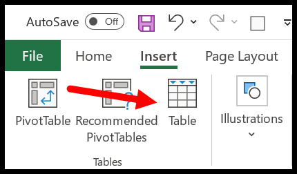
To apply Excel table to data you can go to Insert Excel Table or you can also use the shortcut key Control + T. When you refer to this data in a table, every time you update this data you need to change the reference.

Why? Because the range address of the data changes every time you update it. The best example I can tell you is about using a table while creating a pivot table, you can use a table to update the source range automatically for a pivot table.

6. Conditional Formatting for Better Presentation

Conditional formatting is smart formatting. It helps you to format data based on a condition or logic it helps you to present your data in a better way and also gives you quick insights. To access CF, you need to go to the Home Tab ➜ Style ➜ Conditional Formatting.

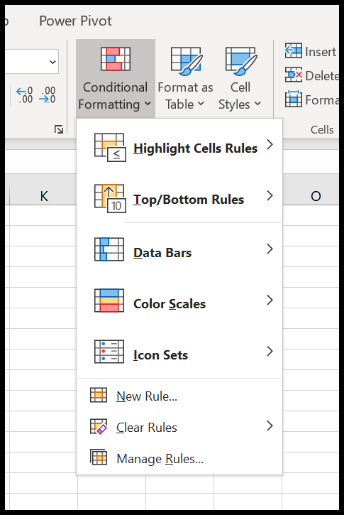
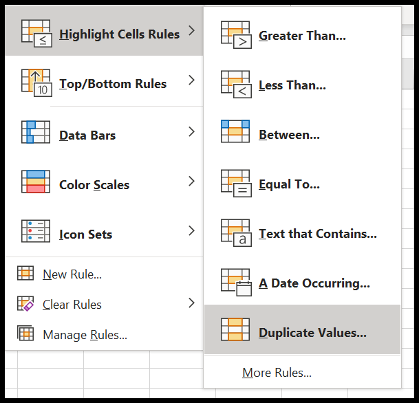
Let’s say you want to highlight duplicate values, with conditional formatting you can do this with a single click. Highlight Cell Rules ➜ Duplicate Values.

Or if you want to highlight the top 10 values, there is an option in conditional formatting called “Top Bottom Rules” which you can use.

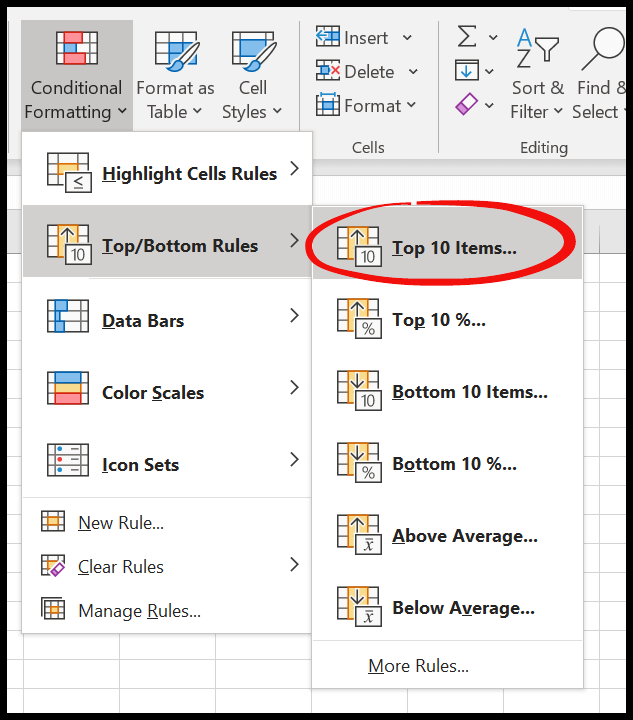
In the same way, you can also apply data bars, color scales, or icon sets to your data.

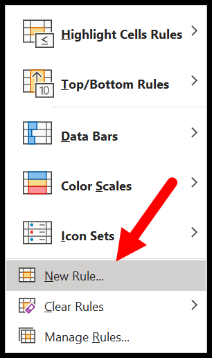
And if you want to create a custom rule to apply CF, click on “New Rule” and you’ll get a dialog box to create a new rule to apply conditional formatting.

Related: Apply Conditional Formatting with Formulas | Apply Conditional Formatting to Pivot Tables

7. Advanced Find and Replace for Smart Users

Apart from normal find and replace there are a few advanced options in Excel to use find and replace. For this, you need to click on the “Options” button and you’ll get a bunch of options down the line. Below I have described them:

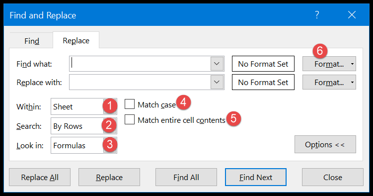
1. Within: You can select the search area for the value. You can select between the active worksheet and the whole workbook.
2. Search: Search through rows or columns.
3. Look in: Look in formulas, values, comments, and notes (This option only works with find, not with find and replace).
4. Match Case: Find and replace a value with a case-sensitive search.
5. Match Entire Content:‌ Match values from the entire value of a cell with the searched value.
6. Format: With this option, you can search a cell based on its formatting. You can specify the formatting or you can use a selection tool to select it from a cell.

Related: Remove Spaces from Cell in Excel

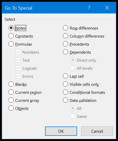
8. GO TO Special for Fast Data Selection

With GO TO special, you can select specific cells just with a single click.

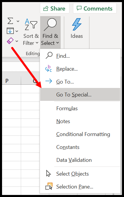
Once you open this, you can see the list of types of cells and objects.

Imagine if you want to select all the cells where you have formulas and those formulas show an error.

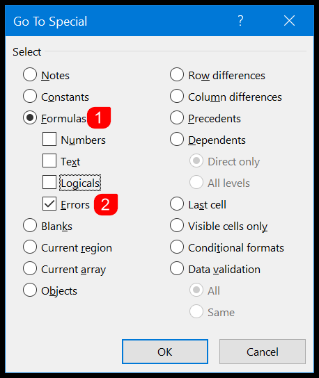
You just need to select the formula and tick mark only errors and click OK and all the cells with formulas with errors will get selected.

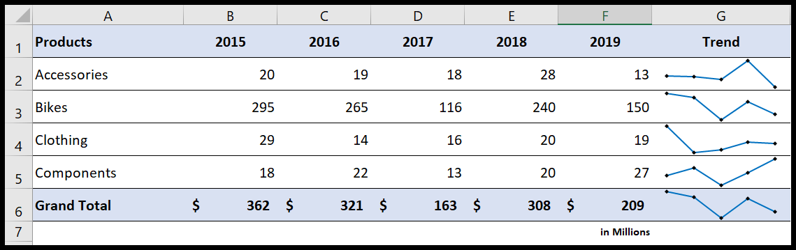
9. Use Sparklines for Tiny Charts

As an accountant, you need to deal with a lot of financial data in tabular form, and sometimes for the end-user, these kinds of data take longer to understand.

But with sparklines, you can make it easily digestible by creating tiny charts. In the below example, I have product-wise and year-wise data and at the end of the rows, I have small charts which I have added by using sparklines.

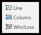
There are three different types of sparklines that you can use:

• Line
• Column
• Win/Loss

To add a sparkline you simply need (Insert Tab ➜ Sparklines) and select the type which you want to insert.

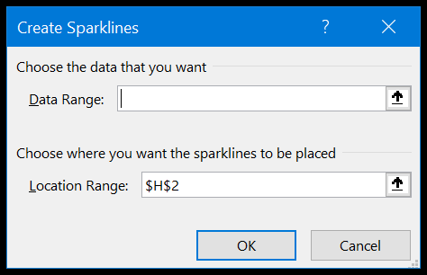
Once you click on the type, you’ll get a dialog box where you need to select the date range, and then you need to specify the destination of the cell for the sparkline. Once you insert it, there are multiple ways to customize it. Simply click on the cell and go to Sparkline.

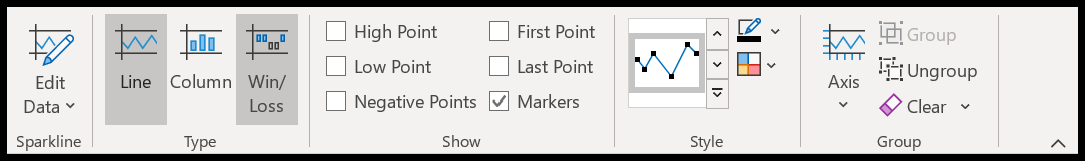
• You can add and remove markers and add high-low points.
• You can change the color of the marker and the line.
• You can also change the type of sparkline in your work.

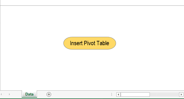
10. Data Analysis with Pivot Table

A pivot table is the most important tool when it comes to data analysis in Excel. You can create a pivot table to create instant financial reports and account summaries of a large set of data. Well, creating a pivot table is easy.

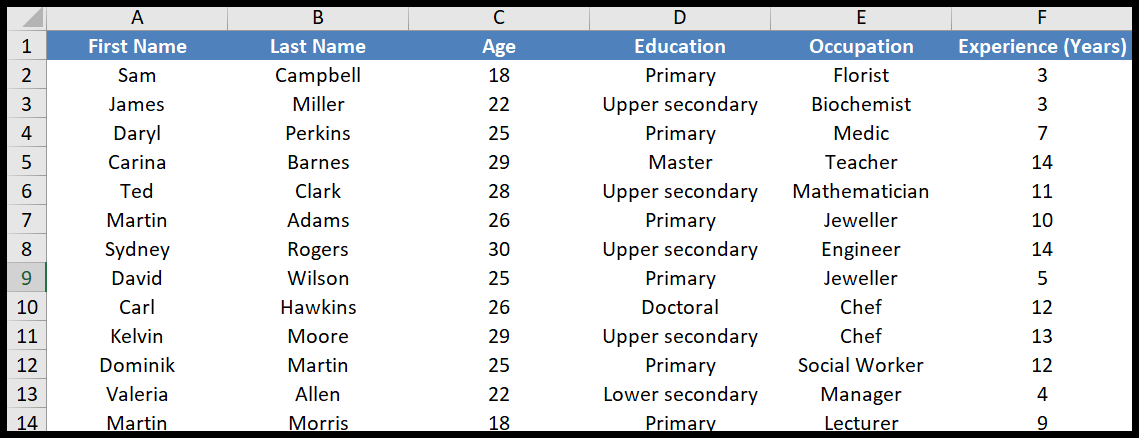
You need to have source data just like I have in the below example, but make sure there shouldn’t any blank rows-columns.

• Now, go to the Insert Tab and click on the insert pivot table.

  

• It will show you a dialog box to define the source data range but as you have already selected the data it takes it automatically.

  

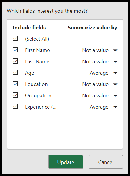
• Once you click OK, you will have a sidebar just like below where you can define the rows, columns, and values for the pivot table. You can simply drag and drop.
• So now, add “Age” to the rows, “Education” to the column, and “First Name” to the values.

  

• In the end, once you define all, you’ll have a pivot chart like below.

  

11. Take the Help of Idea Button

The idea button is a new feature introduced by Microsoft in Excel. The idea behind this button: It can analyze the data with a single click and recommends all the possibilities.

• Category Pivot Table and Charts
• Trendline Charts
• Frequency Distribution Charts

Here’s how to use it:

1. Once you are ready with your data click on the IDEA button (Home Tab ➜ Ideas ➜ Ideas).

   

2. It will instantly show you the side pane and with all the recommendations.

   

3. You can simply click on “Insert” to insert your preferable chart or pivot.

   

There’s also an option to specify the fields which are important and you want the IDEA button to make a recommendation based on those.

12. Use Drop Down List for Fast Data Entry

Accountants need to deal with a lot of data entry work. In that case, it’s important to work with ease and speed. DROP DOWN list gives you both. You can specify multiple options in a drop-down to select which can save you time to enter a value manually.

Follow the below steps:

• First, select the cell where you want to add a drop-down and then go to the Data Tab ➜ Data Tools ➜ Data Validation ➜ Data Validation.

• Now, in the data validation dialog box, select the list from the “Allow” dropdown.
• After that, you need to select the range where you have the values you want to add in the drop-down list or you can also enter them directly, using a comma (,) to separate each value.

• In the end, click OK.

You have a total of 8 different ways to create a drop-down and apart from that, you can also create a cell message and an alert message for a cell.

13. Using Comments and Notes for Audit

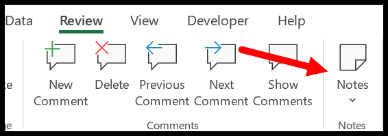
Comments and Notes can be super useful when it comes to auditing reports. Well, both of these are equally useful, but there is one plus point with the comments, you can create a conversation. To add a comment, go to the Review Tab ➜ Comments ➜ New Comment.

And when you enter a comment, it looks like the below example where it says “Start a Conversation”.

Now when you type your comment and hit the enter button and Excel creates a thread where you or anyone (if you share this file with others or use co-authoring) can add their comments.

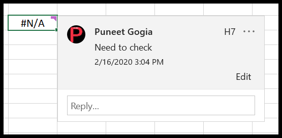
You can navigate to comments with the “Previous” and “Next” buttons and you can also see all the comments on the side pane.

And just next to the comments, there’s a button to add a note. Notes are the compatible version of notes and you can also convert all the notes into comments.

14. Use Named Ranges in Calculations

In financial data, you do have a lot-specific data which you use frequently and a named range can be super useful for that.

Let me show you an example. Imagine you have a discount rate (11%) that you use frequently.

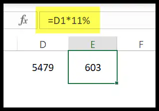
So instead of using the hard value everywhere you can create a named range of that rate and use it in all the formulas.

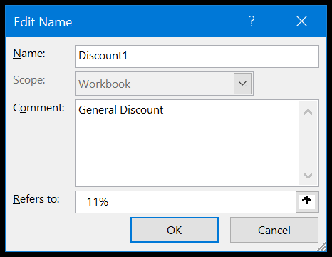
• First, go to the Formula Tab ➜ Defined Names ➜ Define Name.

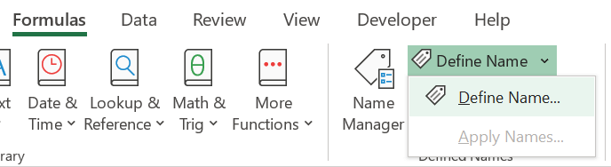
• In the dialog box, you need to enter the following:
  1. Name of the range: Discount1
  2. Scope: Workbook
  3. Comment: General Discount
  4. Refers to: You can refer to a range of input values.

• In the end, click OK.

Now you can use this named range where ever you want to use the discount just by entering “Discount1”.

And if you want to update the rate of discount you simply need to edit the value from the define name dialog box.

15. Functions for Accountants

Excel has a whole bunch of functions (See this:‌ Excel Functions List) and below you have the top functions for accountants:

• ABS: This function converts a number (negative to positive) into an absolute number.
• SUMIFS: With this function, you can sum values from an array using multiple conditions.
• AVERAGEIFS:‌ With this function, you can average values from an array using multiple conditions.
• COUNTIFS: With this function, you can count values from an array using multiple conditions.
• SUMPRODUCT: This function calculates the products of two or more arrays and then returns the sum of those products.
• EOMONTH: It returns the last day of a future or a past month using the number you provide.
• DATEDIF: It returns the number of days between two days using different parameters (days, months, or years).
• FV: It calculates the future value of an investment using constant payments and a constant rate of interest.
• Other Functions: String (Text)

16. Formulas for Accountants

A formula is a combination of two or more Excel functions to calculate a specific value. Once you learn to use functions you can be able to create basic as well as complex formulas. Below is a list of some of the most useful accounting formulas.

1. Add Month to a Date
2. Add Years to Date
3. Add-Subtract Week from a Date
4. Compare Two Dates
5. Convert Date to Number
6. Count Years Between Two Dates
7. Get Day Name from a Date
8. Get the Day Number of the Year
9. Get the End of the Month Date
10. Get the First Day of the Month
11. Get Month from a Date
12. Get Quarter from a Date
13. Get Total Days in a Month
14. Get Years of Service
15. Months Between Two Dates
16. Years Between Dates
17. Separate Date and Time
18. Count Between Two Numbers
19. Count Blank (Empty) Cells
20. Count Cells Less than a Particular Value
21. Count Cells Not Equal To
22. Count Cells That Are Not Blank
23. Count Cells with Text
24. Count Greater Than 0
25. Count Specific Characters
26. Count the Total Number of Cells
27. Count Unique Values
28. OR Logic in COUNTIF/COUNIFS
29. Sum an Entire Column or a Row
30. Sum Greater Than Values using SUMIF
31. Sum Not Equal Values (SUMIFS)
32. Sum Only Visible Cells
33. Capitalize First Letter
34. Change Column to Row
35. Concatenate with a Line Break
36. Horizontal Filter
37. Reverse VLOOKUP
38. Average Top 5 Values
39. Compound Interest
40. Cube Root
41. Percentage Variance
42. Simple Interest
43. Square Root
44. Weighted Average
45. Ratio
46. Square a Number
47. #DIV/0 Error
48. #SPILL! Error
49. #Value Error
50. Ignore All the Errors

17. Excel Charts for Accountants

Even if you work more with finance and accounts data, you do need to present it to others. The best way for this is by using charts, and Excel gives you a full range of charts to insert.

• Line Chart: It is best to show a trend over some time with a line.

• Area Chart:‌ An area chart is a line chart where space to the X-axis is filled.

  

• Column Chart: It can be used to compare different sets of values using data bars.

  

• Bar Chart: It’s a horizontal column chart and useful if you have long data bars.

  

• Pie Chart: With a pie chart, you can present a share of multiple categories as a whole.
• Donut Chart: It’s a pie chart with a blank at the center.

  

• Advanced Excel Charts
• Add Horizontal Line to Excel Chart
• Add Vertical Line to Excel Chart
• Copy Chart Format
• Interactive Charts

18. Visual Basic for Applications

As an accountant, you need to create a lot of reports and with VBA‌ you can automate all those reports that you usually create manually. The best example is, using a macro to create a pivot table.

You need to spend some good time learning VBA‌ but the good news is it’s easy to learn:

• 100 Ready to use Codes
• Run a Macro
• Personal Macro Workbook
• Record a Macro
• Visual Basic Editor
• Objects

19. Take the Help of Power Query

If you deal with a lot of inconsistent data, which I’m sure you do, then you need to learn the power query. Why? With the power query, you can write queries that can work in real-time. Here are some examples:

• Combine Excel Workbooks
• Unpivot Data
• VLOOKUP using Power Query

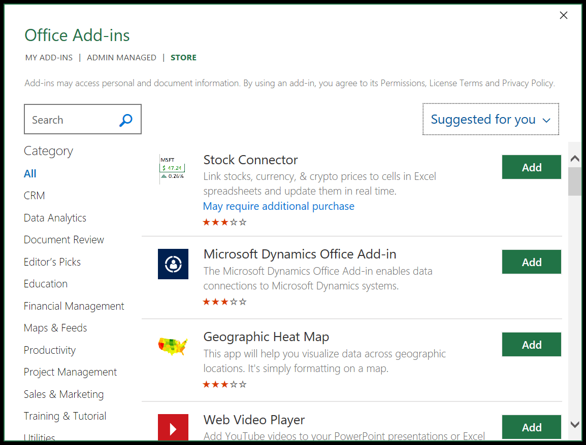
20. OFFICE‌ Add-Ins

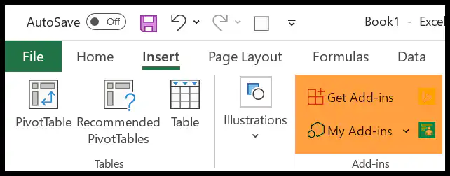
If you use Excel 2013 or a later version, you can access the OFFICE ADD-IN store where you can find a lot of add-ins to increase the functionality of Excel.

It’s on the Insert Tab ➜ Add-Ins ➜ Get Add-Ins and you have thousands of add-ins to install (third party).