

To hide an error inside a formula, wrap it in IFERROR: =IFERROR(A2/B2,"") shows a blank instead of #DIV/0!, and =IFERROR(VLOOKUP(A2,D:E,2,0),"Not found") replaces #N/A with your own text.
IFERROR catches every error type, which is convenient but also means a genuine #REF! from a deleted column gets hidden along with the expected one — use =IFNA(VLOOKUP(...),"Not found") when you only want to trap “not in the list” and still see real problems.
That distinction matters more than it sounds: hiding an error is not fixing it, and a suppressed #REF! silently reports a wrong number.
If you only want to remove the green triangle in the corner of the cell rather than change the result, that’s a separate thing — click the warning icon and choose Ignore Error, or turn the checks off entirely under File → Options → Formulas → uncheck Enable background error checking.
To keep the values visible on screen but blank on a printout, use Page Layout → Print Titles → Sheet → Cell errors as: blank.
In Excel, to ignore all the errors that you get while using formulas, you can use an error-handling function. You can wrap your original formula with an error-handling function that shows a meaningful result when an error occurs. Other than that, you can use the ignore error option as well that you have in Excel.
In this tutorial, we will learn some of the most useful methods for ignoring errors or handling them in a way that will not affect the data’s result. In the end, we will also look at the reasons that cause errors in formulas.
Using IFERROR to Ignore Errors and Replace it with a Meaningful Message
The easiest way to deal with errors is to use the IFERROR function. It allows you to replace error values (like #DIV/0!, #N/A, etc.) with a value you choose, such as zero, a blank cell, or a custom text message.
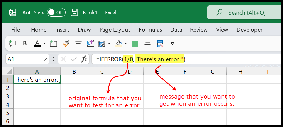
In this function, you have two arguments to define. The first is the value (or formula) that you want to test for an error, and the second is the value that you want to get if an error occurs.

In the following example, you can see we have used the same formula, but we have wrapped it in IFERROR, and it has returned the value that we have defined.

=IFERROR(1/0,"There's an error.")
- Calculation Part (1/0) – This tries dividing 1 by 0. In mathematics, dividing by zero is undefined and will result in an error. In Excel, this specific division will generate a #DIV/0! error.
- IFERROR Function – In the first argument (1/0), Excel first attempts to divide. And then the second argument (“There’s an error.”), this is the value that Excel should return if the first argument results in an error.
You can also use a formula like below, which gives you a 0 instead of a text message, so other formulas that use this cell in a calculation keep working.
=IFERROR(1/0,0)
Just keep in mind that IFERROR hides every type of error. If a formula breaks because of a typo in a function name (#NAME?) or a deleted cell (#REF!), IFERROR hides that too, and you might not notice the problem. So use it when you know which error to expect.
IFNA Function to Ignore #N/A Error
If you specifically want to ignore the #N/A error and replace it with a meaningful message, then you can use the IFNA function (Excel 2013 and later) that only deals with the #N/A error. This function also has two arguments that you need to define.
As you can see in the following example, we have the error in cell D1 which comes from the VLOOKUP function.

Now to deal with this error, you can use the IFNA (you can also use IFERROR with the VLOOKUP, but we will use IFNA here).

The formula looks like this. It returns “Not Found” when VLOOKUP can’t find the value, but any other error still shows up, so you can spot real problems:
=IFNA(VLOOKUP(C1,A1:B10,2,FALSE),"Not Found")
Ignoring Error from the Options
When you get an error in a cell, Excel gives you an option along with that cell where you can use the “Ignore Error” option. As you can see in the following example, you have a #DIV/0! error in cell A1.
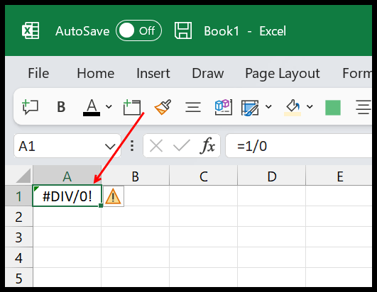
Now with cell A1, you have a small icon on the right side, and when you click on this icon, it gives you a list of options. And from these options, you can select the “Ignore Error” option.

And once you click on this option, Excel stops marking that cell as an error cell. Note that this only removes the green triangle and the warning icon; the cell still shows #DIV/0!. To replace the error value itself, use IFERROR or IFNA.

Turn ON-OFF Error Checking Options
Apart from that, you can use the error-checking options in Excel Options to stop Excel from flagging errors (the green triangles).
The Error Checking Options let you manage how Excel flags formula errors. You can also open them from File ➜ Options ➜ Formulas.
These settings allow you to control how Excel flags potential errors in your worksheets. Here’s how you can access and configure the Error Checking Options:

When you click on “Error Checking Options”, you get the Excel Options dialog box, from where you can turn on and off the error checking options.

From these options, you need to un-tick the “Enable background error checking” to turn off the error checking options. The moment you do this, it turns off error checking for the entire Excel application. Again, the error values stay in the cells; only the flags go away. To stop flagging only error values, untick “Cells containing formulas that result in an error” under Error checking rules instead.
Why Errors Occur in Excel Formulas
Errors occur in Excel formulas for various reasons, typically indicating something is wrong with how a formula is written or the data it references. Understanding these errors can help troubleshoot and refine formulas to ensure they work correctly. Here are some common reasons why errors might occur:
- Division by Zero (#DIV/0!): This happens when a formula tries to divide a number by zero. For example, =A1/B1 will result in this error if B1 contains zero.
- Non-Existent Cell Reference (#REF!): If your formula refers to a cell that doesn’t exist, perhaps because it was deleted or the reference is incorrect, you’ll get this error. This often occurs after deleting columns or rows on which a formula depends.
- Invalid Formula (#VALUE!): This error appears when a formula has the wrong type of argument. For example, adding a numeric value to a text string.
- Name Error (#NAME?): If Excel doesn’t recognize text in a formula, it will display this error. It often happens when function names are misspelled or named ranges are not defined.
- Null Value (#NULL!): This error is not common and occurs when you specify an intersection of two areas that do not intersect. It’s often caused by a misused space character in formulas that implicitly intersect multiple ranges.
- Not Available (#N/A): This error means that a value is not available to a formula. You see it most often with lookup functions like VLOOKUP when the lookup value is not found.
- Number Error (#NUM!): This occurs when a formula or function contains invalid numeric values. It’s a common issue with functions that require strict numeric input, such as the square root of a negative number.
- Getting Data (#GETTING_DATA): This is a temporary message seen in Microsoft 365. It indicates that Excel is currently fetching data required by a formula but hasn’t completed the task yet.
Newer versions of Excel have a few more errors, like #SPILL! (a dynamic array formula has no room to spill) and #CALC! (for example, FILTER finds nothing). Each error tells you how your formula is written and what might need to be fixed. Using the methods mentioned above, you can make sure your formulas work correctly.
Do I Really Need to Ignore Errors?
As we have discussed, ignoring errors in Excel formulas using the IFERROR function or other methods can offer several benefits, especially when preparing complex data or reports for presentation.
- Readability: By replacing errors with custom text or zero, data becomes easier to read and understand. This is particularly helpful when presenting data to people who may not be familiar with Excel’s error codes.
- Prevent Further Errors: Errors in one part of the data can also cause other formulas that depend on those cells to fail. Handling these errors can prevent such cascading errors, so more formulas in your worksheet work correctly.
- Custom Error Responses: You can provide specific messages or values that are more meaningful in the context of your data. For example, instead of showing #DIV/0!, showing “No data” or “Not applicable” can be more informative.
Ignore Errors While Summing or Averaging
If a range has an error, SUM, AVERAGE, MAX and other functions on that range return the error too. Instead of fixing each cell, use AGGREGATE (Excel 2010 and later). The first argument picks the function (9 for SUM, 1 for AVERAGE), and 6 tells it to ignore error values:
=AGGREGATE(9,6,A1:A10)
=AGGREGATE(1,6,A1:A10)
Hide Errors with Conditional Formatting
If you can’t change the formulas, you can hide the errors visually. Select the range, go to Home ➜ Conditional Formatting ➜ New Rule ➜ Use a formula to determine which cells to format, enter the formula below (for a range that starts at A1), and set the font color to white:
=ISERROR(A1)
The error is still in the cell, so formulas that refer to it still get the error. Use ISERR instead of ISERROR if you want to keep #N/A visible.
Ignore Errors When Printing or in a Pivot Table
- Printing: go to Page Layout ➜ Page Setup (the small arrow), open the Sheet tab, and set “Cell errors as” to <blank>, — or #N/A.
- Pivot table: right-click the pivot table ➜ PivotTable Options ➜ Layout & Format, tick “For error values show”, and enter what you want to see (or leave it empty).
Frequently Asked Questions
What is the difference between IFERROR and IFNA?
IFERROR replaces every type of error. IFNA replaces only #N/A and lets other errors, like #DIV/0! or #REF!, show up. IFNA is safer for lookup formulas.
Does Ignore Error remove the error from the cell?
No. It only stops Excel from flagging the cell with the green triangle. The cell still shows the error value until you fix the formula or wrap it in IFERROR.
How do I sum a range that has errors?
Use AGGREGATE with option 6, which ignores the error values:
=AGGREGATE(9,6,A1:A10)
Written by
Puneet Gogia
Microsoft MVP — Excel · Founder, Excel Champs
Twelve years of teaching Excel, and a decade before that using it as a data analyst. Every tutorial here is written from a file I actually built.