#VALUE! Error in Excel (Understanding and Fixing)

In Excel, the #VALUE! error appears when a formula gets the wrong type of value, like text where it expects a number. Let’s say you want to add the numbers from two cells, but the second cell has text instead of a number. Excel can’t add a number and text, so the formula returns #VALUE!.

In this tutorial, you’ll learn what causes the #VALUE! error and how to fix it in your formulas.

Steps to Fix #VALUE! Error in Excel

Here are a few points and steps you can follow to fix the value error:

1. Incorrect Data Types: First, check the data type. If you’re adding or multiplying with operators like + and *, the cells should contain numbers, not text. Dates are fine, because Excel stores dates as numbers. Text that looks like a number (like “25”) usually works too, because Excel converts it, but text like “N/A” or “25 kg” doesn’t. If you can’t clean the data, use SUM and PRODUCT instead of + and *, because they skip text.
2. Invalid Argument Values: Check that each argument has a value the function can accept. For example, MID returns #VALUE! when the start position is less than 1, and FIND returns #VALUE! when it can’t find the text you’re looking for. But asking MID for the 25^th character of a 20-character text doesn’t give an error. MID just returns empty text.
3. Dimension of the Arrays: After that, check the sizes of the ranges you refer to. In functions like SUMPRODUCT and SUMIFS, if one range has ten cells and the other has 12, the formula returns #VALUE!.
4. Array Formula Issues: In Excel 2019 and earlier, you need to press Ctrl + Shift + Enter instead of Enter to enter an array formula. If you press only Enter, the formula can return #VALUE!. In Excel 365 and Excel 2021, Enter is enough.
5. Error Already Exists: Check whether any cell your formula refers to already shows #VALUE!. Most formulas pass that error along, so fix the first cell with the error and the others usually clear up.
6. Spaces or Non-visible Characters: Sometimes, cells have invisible characters like spaces. TRIM removes extra spaces and CLEAN removes non-printing characters, but a cell with nothing but a space needs a different fix (see the example below).

These are the first checks to run when you see the error. Now, let’s look at a few real examples.

#VALUE! Error With SUMPRODUCT

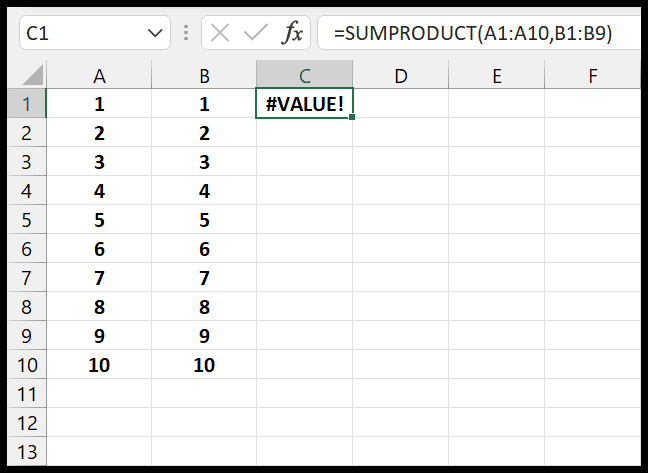
In the following example, I have used the SUMPRODUCT function. The first array has ten cells, but in the second array, I mistakenly referred to B1:B9, which has only nine cells. SUMPRODUCT needs all the arrays to be the same size, so it returns #VALUE!. To fix it, change the second range so it also has ten cells.

The same rule applies to SUMIFS, AVERAGEIFS and COUNTIFS: every range must be the same size, or you get #VALUE!. SUMIF and AVERAGEIF are different. When the ranges don’t match, they don’t return an error. They quietly resize the sum or average range to match the first range, starting from its top-left cell. So you won’t see #VALUE! there, but it’s still worth checking that your ranges line up.

#VALUE! Error While Working with Dates

In the following example, the date in cell A1 is stored as text, in a format Excel doesn’t recognize as a date. When you use it in a calculation, the formula returns #VALUE!.

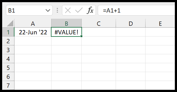
That’s because Excel stores real dates as numbers. A date stored as text is just text to Excel, even though you can read it as a date. A quick clue: text dates sit on the left side of the cell, while real dates line up on the right.

If the text is in a date format Excel recognizes, you can convert it with DATEVALUE or VALUE:

=DATEVALUE(A1) + 1
=VALUE(A1) + 1

Both return the date as a serial number, so format the result cell as a date to see it as one. If the text isn’t in a format Excel recognizes, DATEVALUE returns #VALUE! as well, and you need one of the fixes below.

If dates are entered in a format that doesn’t match your system’s regional settings, Excel may not recognize them as valid dates. For example, if you enter dates as DD/MM/YYYY but your system uses MM/DD/YYYY, a date like 25/12/2024 stays as text and returns #VALUE! in a calculation. A date like 05/12/2024 is even trickier: it doesn’t give an error, but Excel reads it as May 12 instead of December 5. Changing the cell’s number format won’t fix this, because a format doesn’t turn text into a date. You need to convert the text, using one of the two methods below.

To rebuild a DD/MM/YYYY text date, use the DATE function like this. It works when the day and month always have two digits and the year has four.

=DATE(RIGHT(A1,4),MID(A1,4,2),LEFT(A1,2))

To convert a whole column at once, select it and go to Data > Text to Columns. Click Next twice, choose Date under Column data format, pick the order your dates use (like DMY), and click Finish.

#VALUE! When Including a Space Value in a Calculation

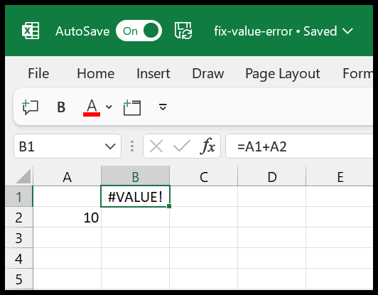
In the following example, when I tried to add cells A1 and A2, I got the #VALUE! error. That’s because cell A1 contains a space, even though it looks empty.

To Excel, a space is text. So when the + operator meets a cell with a space where it expects a number, the formula fails and returns #VALUE!. A truly empty cell doesn’t cause this, because Excel treats it as 0.

Now, to fix this: If the space is in a single cell, select A1 and press Delete, and the formula works. If a cell has a number with extra spaces around it (like ” 25 “), TRIM or VALUE can clean it inside the formula:

=TRIM(A1) + A2
=VALUE(A1) + A2

These two only help when there’s a number in the cell. If A1 has nothing but a space, TRIM returns empty text and VALUE can’t convert it, so both formulas still return #VALUE!. In that case, use SUM instead, which skips text:

=SUM(A1,A2)

To clear spaces from a whole range of numbers, select it, press Ctrl+H, type a single space in Find what, leave Replace with empty and click Replace All. Only do this on cells that hold numbers, because it also removes the spaces between words in text.

Data copied from websites often has non-breaking spaces (character 160), which TRIM doesn’t remove. Use SUBSTITUTE for those. For other hidden characters, like line breaks, use CLEAN.

=SUBSTITUTE(A1,CHAR(160),"")+A2

Read Also – Remove Extra Spaces in Excel

Problem with Array Formulas

One lesser-known cause of the #VALUE! error is giving a range to a formula that expects a single value. This mostly happens in Excel 2019 and earlier.

For example, in Excel 2019 and earlier, if you enter a formula like =A1:A5 + 1 with just Enter (instead of Ctrl + Shift + Enter), Excel tries to pick one value from the range, from the same row as the formula. In a row outside rows 1 to 5, there’s nothing to pick, so it returns #VALUE!. In Excel 365 and Excel 2021, the same formula spills the five results into the cells below instead.

This is easy to miss when you accidentally select a range instead of a single cell. In older versions, the formula may even work in some rows (where it picks the value from the same row) and fail in others, so it looks like the data is the problem.

To avoid this error, check that every reference points to a single cell where the formula expects one, or enter the formula as an array formula.

#VALUE! Error in Other Functions

Some functions return #VALUE! for their own reasons, even when the data types look right:

• FIND and SEARCH: return #VALUE! when they can’t find the text. To get TRUE or FALSE instead, wrap them in ISNUMBER (example below this list).
• MID, LEFT and RIGHT: return #VALUE! when the number of characters is negative. MID also returns it when the start position is less than 1.
• VLOOKUP: returns #VALUE! when the column number is less than 1, or when the lookup value is longer than 255 characters. For long lookup values, use INDEX and MATCH instead.
• DATEVALUE and DAYS: return #VALUE! when a date is text that Excel can’t read as a date.
• SUMIF and SUMIFS: return #VALUE! when they refer to a range in another workbook that’s closed. Open that workbook and press F9 to recalculate.

For example, this formula returns TRUE when A1 contains “abc” and FALSE when it doesn’t, instead of #VALUE!:

=ISNUMBER(SEARCH("abc",A1))

How to Find What’s Causing the #VALUE! Error

When a long formula returns #VALUE!, Excel can show you which part breaks it.

1. First of all, select the cell with the error and go to Formulas > Evaluate Formula (in the Formula Auditing group).
2. After that, click Evaluate again and again. Excel works through the formula one part at a time, and the step that turns into #VALUE! shows you the problem. A hidden space shows up as ” “.
3. In the end, check any suspicious cell with ISTEXT, which returns TRUE for text, and LEN, which counts its characters (formulas below this list). A cell that looks empty but has a length above 0 has a hidden space or character in it.

=ISTEXT(A1)
=LEN(A1)

To list every #VALUE! error on the sheet, press Ctrl+F, click Options, set Look in to Values, type #VALUE! in Find what and click Find All. Excel lists every matching cell, and you can click a result to jump to it.

Replace the #VALUE! Error with 0 or a Blank

If you’ve checked the formula and still want to hide the error, wrap it in IFERROR:

=IFERROR(A1+A2,0)

Use “” instead of 0 to show a blank cell. Keep in mind that IFERROR hides every error, not just #VALUE!, so use it only once you’re sure the formula itself is right. For more ways to handle errors, see Ignore All the Errors in Excel.

Frequently Asked Questions