Last Updated:
Quick formula reference
Just need the formula? Here's each method in one line — copy, adapt, done.
=XLOOKUP(lookup_value, lookup_range, return_range)
=XLOOKUP(D2, B2:B11, A2:A11)
Looks up the value in D2 inside B2:B11 and returns the matching value from A2:A11 (column on the left).
=INDEX(return_range, MATCH(lookup_value, lookup_range, 0))
=INDEX(B2:B11, MATCH(E3, A2:A11, 0))
MATCH finds the position of E3 in A2:A11, then INDEX returns the value from that same position in B2:B11.
=LOOKUP(lookup_value, lookup_range, return_range)
=LOOKUP(E3, A2:A11, B2:B11)
Simplest syntax. Requires sorted data — for unsorted data, use =LOOKUP(2, 1/(A2:A11=E3), B2:B11).
=VLOOKUP(lookup_value, CHOOSE({1,2}, lookup_range, return_range), 2, 0)
=VLOOKUP(E3, CHOOSE({1,2}, A2:A11, B2:B11), 2, 0)
CHOOSE virtually swaps the columns so VLOOKUP can look to the left. May need Ctrl + Shift + Enter in Excel 2019 and earlier.
=FILTER(return_range, lookup_range=lookup_value)
=FILTER(A2:A11, B2:B11=E3)
Returns every matching row, not just the first. Results spill into adjacent cells automatically.
=XLOOKUP(lookup_value, lookup_range, return_range, , 0, -1)
=XLOOKUP(D2, B2:B11, A2:A11, , 0, -1)
The -1 tells XLOOKUP to search from last to first — returns the last occurrence instead of the first.
A reverse VLOOKUP in Excel means looking up a value from a column that sits to the left of your lookup column, something the standard VLOOKUP function cannot do on its own. It's also commonly searched as VLOOKUP to the left, VLOOKUP backwards, or right to left VLOOKUP.
The reason VLOOKUP can't handle this natively is simple: it always searches the first column of the range you give it and returns a value from a column to the right. So if your lookup column is on the right side of the data and the value you want is on the left, VLOOKUP fails.
The good news, there are four reliable ways to do a reverse lookup in Excel, and at least one works in every version of Excel ever released. In this guide, you'll learn:
- Method 1 — XLOOKUP Recommended Excel 365 / 2021+
- Method 2 — INDEX and MATCH All Excel versions
- Method 3 — LOOKUP function All Excel versions
- Method 4 — VLOOKUP with CHOOSE All Excel versions
You'll also find a comparison table, a troubleshooting section, a sample workbook, and answers to the most-asked questions.
Quick comparison — Which reverse VLOOKUP method to use?
Pick the method that matches your Excel version. Click any row to jump to its tutorial section.
Method |
Excel version |
Best for |
Difficulty |
|---|---|---|---|
XLOOKUP
Recommended
|
365, 2021, Web, Mac 2021+ |
Most users — simplest syntax, handles every direction |
Easy |
All versions |
Older Excel (2019, 2016) and large datasets |
Medium |
|
All versions |
Quick lookups when data is sorted |
Easy |
|
All versions |
When you must use VLOOKUP (legacy templates) |
Advanced |
1 Reverse VLOOKUP with XLOOKUP Recommended
XLOOKUP is the modern replacement for VLOOKUP and HLOOKUP, and it handles a reverse lookup natively — no tricks, no helper columns. It can search a range and return a value from any direction (left, right, up, or down), which makes it the simplest way to do a VLOOKUP to the left.
Syntax
=XLOOKUP(lookup_value, lookup_array, return_array, [if_not_found], [match_mode], [search_mode])
- lookup_value — the value you want to search for.
- lookup_array — the range where Excel will search for the value.
- return_array — the range from which Excel returns the matching value (this can sit to the left of the lookup_array — that's what makes it a reverse lookup).
- [if_not_found] — the value to return if no match is found. Optional.
- [match_mode] — 0 for exact match, -1 for exact or next smaller, 1 for exact or next larger, 2 for wildcard. Optional, defaults to 0.
- [search_mode] — 1 for first-to-last, -1 for last-to-first. Optional, defaults to 1.
Example
In the example below, you have a list of Employee Names in column A and Employee IDs in column B. You need to look up an Employee ID and return the matching Name from the column on the left.

Here's the formula:
=XLOOKUP(D2,B2:B11,A2:A11,"Not Found",0,1)
- D2 — the Employee ID you're searching for.
- B2:B11 — the lookup column (Employee IDs).
- A2:A11 — the return column (Names) — sitting to the left of the lookup column.
- "Not Found" — what to display if the ID doesn't exist.
- 0 — exact match.
- 1 — search from first to last.
How the formula works
XLOOKUP takes the value in cell D2 and searches for it inside the range B2:B11. The moment it finds a match, it returns the value from the same row position in A2:A11 — even though A2:A11 is to the left of the lookup column. If the ID isn't found, it shows "Not Found" instead of the standard #N/A error.
Unlike VLOOKUP, XLOOKUP doesn't care which column comes first. The lookup_array and return_array are independent — that's the entire reason it solves the reverse-lookup problem so cleanly.
Compatibility
When to use this method
Use XLOOKUP if you're on Excel 365, Excel 2021, or any newer version. It's the cleanest, fastest, and most readable way to do a reverse lookup. If you're on Excel 2019 or older and you see #NAME? when you type XLOOKUP, jump to Method 2 (INDEX-MATCH) instead.
2 Reverse VLOOKUP with INDEX and MATCH
Before XLOOKUP existed, the INDEX-MATCH combination was the standard solution for reverse lookups — and it still is for anyone using Excel 2019 or earlier. It works in every version of Excel, handles large datasets faster than VLOOKUP, and is more flexible than XLOOKUP in some edge cases.
The trick is simple once you see it:
MATCH tells INDEX the position (cell number) of a value in a column or row, and INDEX returns the value from that position.
Think of it this way — MATCH is the undercover agent who finds the criminal, and INDEX is the cop who arrests that criminal afterward.

Syntax
Here's the syntax of the INDEX function on its own:
=INDEX(array, row_num, [column_num])
- array — the column (or range) you want to return a value from.
- row_num — the row position of the value inside that array.
- [column_num] — the column position (only needed if the array has multiple columns). Optional.
The row_num argument is the missing piece. If you enter 4, INDEX returns the value from the 4th row of the array. The whole INDEX-MATCH trick comes down to one move:
Replace the row_num argument of INDEX with a MATCH formula.
MATCH looks up your value in the lookup column and returns its position number. INDEX then uses that position to pull the matching value from the return column — even when the return column is to the left of the lookup column.
Example
Below, you have a list of cities in column A and the names of employees working in those cities in column B. The goal is to look up the employee name working in Mumbai — meaning column A is the lookup column and column B is the return column.

Here's the formula:
=INDEX(B2:B11,MATCH(E3,A2:A11,0),0)
- B2:B11 — the return column (employee names).
- E3 — the city you're looking up (Mumbai).
- A2:A11 — the lookup column (cities).
- 0 — exact match.

How the formula works
Let's break the formula into two parts.
Part 1 — MATCH finds the position The MATCH function looks for the value "Mumbai" inside the cities column (A2:A11) and returns 5 — because Mumbai is in the 5th cell of that column.
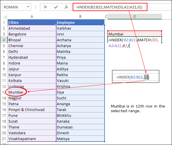
Part 2 — INDEX returns the value INDEX now knows it needs to return the value from the 5th cell of the employee names column (B2:B11). The 5th cell contains "Siya" — so that's the result.

That's the full mechanic — MATCH locates the row, INDEX delivers the value. Because the two functions are independent, the lookup column and the return column can sit in any order. That's what makes INDEX-MATCH a reverse VLOOKUP.
Compatibility
When to use this method
Use INDEX-MATCH if you're on Excel 2019 or older (where XLOOKUP doesn't exist), if you're sharing your file with people who might be on older versions, or if you're working with very large datasets where INDEX-MATCH typically outperforms VLOOKUP. It's the most universally compatible reverse-lookup method in Excel.
3 Reverse VLOOKUP with the LOOKUP function
The LOOKUP function is the oldest lookup function in Excel — older than VLOOKUP, HLOOKUP, and certainly XLOOKUP. It's also the simplest. Unlike VLOOKUP, LOOKUP doesn't care about column order, which means it can do a reverse lookup with no helper columns and no array tricks.
It comes with one important catch — and we'll cover it in detail in the "How it works" section.
Syntax
LOOKUP has two forms. For reverse lookups, you only need the vector form:
=LOOKUP(lookup_value, lookup_vector, [result_vector])
- lookup_value — the value you want to search for.
- lookup_vector — a single row or column where Excel searches for the value.
- [result_vector] — a single row or column from which Excel returns the matching value. Can be on the left or right of the lookup_vector. Optional — if omitted, LOOKUP returns from the lookup_vector itself.
Example
Using the same dataset from Method 2 — cities in column A and employee names in column B — let's look up the employee working in Phoenix. Cities are the lookup column; names are the return column on the left.

Here's the formula:
=LOOKUP(E3,A2:A11,B2:B11)
- E3 — the city you're looking up (Mumbai).
- A2:A11 — the lookup_vector (cities).
- B2:B11 — the result_vector (employee names).
Notice there's no match-type argument — LOOKUP doesn't need one. The result is "Siya", the same answer you got with INDEX-MATCH and XLOOKUP.
How the formula works
LOOKUP searches the lookup_vector (A2:A11) for the value in E3. When it finds a match, it returns the value from the same position in the result_vector (B2:B11). Because the two vectors are independent ranges, the result column can sit anywhere — left, right, on a different sheet, even non-adjacent.
Important — LOOKUP assumes your lookup column is sorted in ascending order. If it isn't, LOOKUP can return the wrong value without showing any error. This is the single biggest reason INDEX-MATCH and XLOOKUP have largely replaced LOOKUP in modern Excel work.
For unsorted data, there's a workaround using a 1/(condition) pattern that forces an exact match:
=LOOKUP(2,1/(A2:A11=E3),B2:B11)
This formula always returns the correct value even when the data is unsorted, because the 1/(A2:A11=E3) trick creates an array of 1s and #DIV/0! errors, and LOOKUP then finds the last 1 — which is your match.
Compatibility
When to use this method
Use the standard LOOKUP form when your data is genuinely sorted in ascending order — for example, looking up a price band, a tax bracket, or a grade tier. Use the 1/(condition) trick when you need an exact match on unsorted data and you can't (or don't want to) use INDEX-MATCH or XLOOKUP. For most everyday reverse lookups, however, XLOOKUP or INDEX-MATCH are safer choices because they don't carry the sorting risk.
4 Reverse VLOOKUP using VLOOKUP with CHOOSE
This is the classic workaround for situations where you must use VLOOKUP — usually because you're working inside an existing template, following a company standard, or learning Excel before XLOOKUP existed. The CHOOSE function tricks VLOOKUP into thinking the columns are in a different order than they actually are, which lets it look up a value and return a result from the column on the left.
It's clever, it's old-school, and it works in every version of Excel.
Syntax
The pattern combines VLOOKUP with CHOOSE inside the table_array argument:
=VLOOKUP(lookup_value, CHOOSE({1,2}, lookup_column, return_column), 2, 0)
- lookup_value — the value you want to search for.
- CHOOSE({1,2}, lookup_column, return_column) — builds a virtual two-column array where the lookup column comes first and the return column comes second, regardless of where they actually live in your data.
- 2 — tells VLOOKUP to return the value from the second column of the virtual array (which is your return column).
- 0 — exact match.
Example
Using the same cities/employees dataset from Methods 2 and 3 — let's look up the employee working in Mumbai using VLOOKUP, even though the names column sits to the left of the cities column.
=VLOOKUP(E3,CHOOSE({1,2},A2:A11,B2:B11),2,0) entered in Excel returning "Siya" for Mumbai. Same dataset as Methods 2 and 3.
Suggested filename: reverse-vlookup-with-choose-array.png · Max width 680px
Here's the formula:
=VLOOKUP(D3,CHOOSE({1,2},A2:A12,B2:B12),2,0)
- E3 — the city you're looking up (Phoenix).
- CHOOSE({1,2},A2:A11,B2:B11) — virtually places the cities column (A2:A11) as column 1 and the names column (B2:B11) as column 2.
- 2 — return the value from the second virtual column (names).
- 0 — exact match.
The result is "David Wilson" — the same answer as the previous three methods, but achieved using VLOOKUP, which by itself can't look to the left.
How the formula works
VLOOKUP normally fails on a reverse lookup because it requires the lookup column to be the first column of the table_array. CHOOSE solves this by creating a brand-new two-column array in memory — Excel never actually sees your real data layout, just the rearranged version CHOOSE hands it.
The {1,2} argument is the key — it's an array constant that tells CHOOSE to return both values, in that order. So CHOOSE({1,2},A2:A11,B2:B11) returns a 10-row, 2-column virtual table where A2:A11 is column 1 and B2:B11 is column 2.
VLOOKUP then operates on that virtual table exactly as it would on a normal range — searches column 1 (cities), returns the matching value from column 2 (names). The reverse lookup happens silently inside CHOOSE, before VLOOKUP ever runs.
Quick check — in modern Excel (365 or 2021), this formula works as a regular formula. In Excel 2019 and earlier, you may need to enter it as an array formula by pressing Ctrl + Shift + Enter instead of just Enter. If you see #VALUE! in older Excel, that's almost always the cause.
Compatibility
When to use this method
Use VLOOKUP + CHOOSE when you're stuck with a template that already uses VLOOKUP and you can't switch to another function, when you're following a company standard that mandates VLOOKUP, or when you're teaching VLOOKUP and want to show students that even "left lookup" is possible without changing functions. For everyday work where you have a free choice, XLOOKUP or INDEX-MATCH are simpler and easier to read six months later.
5 Reverse VLOOKUP with the FILTER function Excel 365 / 2021
The FILTER function solves a problem that none of the previous four methods can — it returns every matching result, not just the first. If your lookup value appears multiple times in the data and you need all the matches, FILTER is the only clean, single-formula answer in modern Excel.
It's also a reverse-lookup method by default. The return column can sit on either side of the lookup column, and FILTER doesn't care about column order at all.
Syntax
=FILTER(array, include, [if_empty])
- array — the range you want to return values from (this can sit to the left of your lookup column — making it a reverse lookup).
- include — the condition, written as a comparison that returns TRUE or FALSE for each row (e.g.
B2:B11=E3). - [if_empty] — the value to return if no rows match the condition. Optional.
Example
Using the cities/employees dataset from Methods 2, 3, and 4 — this time, imagine three employees work in Mumbai. The previous methods would return only the first name found. FILTER returns all three at once.
=FILTER(A2:A11,B2:B11=E3) entered in Excel returning three employee names spilled vertically into adjacent cells when multiple employees work in Mumbai. Show the blue spill border around the result range.
Suggested filename: reverse-vlookup-with-filter-function.png · Max width 680px
Here's the formula:
=FILTER(A2:A11, B2:B11=E3, "No match found")
- A2:A11 — the return column (employee names) — sitting to the left of the lookup column.
- B2:B11=E3 — the condition (find every row where the city in column B equals the value in E3).
- "No match found" — what to display if nobody matches.
If three employees are based in Mumbai, FILTER spills all three names into the cells below your formula automatically — no need to copy the formula down, no need for Ctrl + Shift + Enter, no helper columns.
How the formula works
FILTER evaluates the include argument for every row in the array and builds a result set containing only the rows where the condition returns TRUE. The output is a dynamic array — Excel automatically sizes the result range to match the number of matches, and updates it in real time when your data changes.
The comparison B2:B11=E3 creates a 10-row array of TRUE/FALSE values. FILTER then returns the corresponding values from A2:A11 only for the rows where the comparison evaluated to TRUE. Because the array (A2:A11) and the condition (B2:B11=E3) are independent, the return column can sit anywhere — to the left, to the right, on another sheet, or in non-adjacent columns.
FILTER with multiple criteria
FILTER handles multi-criteria lookups without any helper columns or array tricks. Multiply conditions together for AND logic, add them for OR logic:
=FILTER(A2:A11, (B2:B11=E3)*(C2:C11="Active"))
This returns names only where the city matches E3 and the status in column C is "Active". For an OR condition, swap the asterisk for a plus sign:
=FILTER(A2:A11, (B2:B11=E3)+(B2:B11=E4))
This returns names where the city matches either E3 or E4. Multi-criteria filtering used to require complex array formulas or helper columns — FILTER collapses it all into a single expression.
Compatibility
When to use this method
Use FILTER when you need more than one match for your lookup value, when you need to apply multiple criteria in a single formula, or when you want the results to update automatically as your source data changes. For a single-match reverse lookup, XLOOKUP is still the simpler choice — FILTER is specifically for the "I need every row that matches" problem. On Excel 2019 or earlier, where FILTER doesn't exist, the equivalent approach uses array formulas combining INDEX, SMALL, and IF — significantly more complex and outside the scope of this guide.
Which reverse VLOOKUP method should you use?
Four methods, plus two bonus tricks — that's a lot of choice. Here's how to pick the right one in under 30 seconds.
Use XLOOKUP. It's the cleanest, most readable, and most flexible method. There's no reason to use anything else unless you're sharing your file with someone on an older Excel version.
Use INDEX-MATCH. It's the universal solution — works in every version, handles any direction, and is faster than VLOOKUP on large datasets. This was the standard reverse-lookup method for two decades for good reason.
Use INDEX-MATCH. If even one person opens your file in Excel 2019 or earlier, XLOOKUP will return #NAME? for them. INDEX-MATCH is the safe choice when you don't control the recipient
Common errors and how to fix them
Reverse-lookup formulas fail in predictable ways. Here are the five errors readers hit most often, what causes each one, and how to fix them.
What it means — Excel searched the lookup column and didn't find your value. The formula is correct; the data isn't matching.
Three most common causes —
- Trailing or leading spaces. "Mumbai " (with a trailing space) is not the same as "Mumbai" to Excel. Wrap the lookup value in TRIM:
=XLOOKUP(TRIM(D2), B2:B11, A2:A11) - Numbers stored as text. If your Employee IDs look like numbers but are formatted as text (or vice versa), the match fails silently. Look for the small green triangle in the corner of the cell — that's Excel telling you the data type is inconsistent.
- The value genuinely doesn't exist. Double-check the spelling and the source range. With XLOOKUP, you can wrap an explicit fallback:
=XLOOKUP(D2, B2:B11, A2:A11, "Not Found")
What it means — The function name itself isn't valid in your version of Excel. For reverse-lookup formulas, this almost always means XLOOKUP or FILTER on Excel 2019 or earlier.
The fix — XLOOKUP and FILTER only exist in Excel 365, Excel 2021, Excel for the web, and Excel for Mac 2021+. If you're on an older version, switch to INDEX-MATCH (Method 2) — it works everywhere and produces the same result. You can check your Excel version under File → Account on Windows or Excel → About Excel on Mac.
What it means — One of your range references is broken — usually because a column or row was deleted, or a sheet was renamed.
The fix — Click into the formula bar and look for any reference that shows #REF! instead of a normal range like A2:A11. Replace it with the correct range. If you copied the formula from a deleted location, you'll need to re-enter the affected cell references manually.
What it means — Excel can't process one of the arguments because of a data-type mismatch — or, very commonly with the VLOOKUP + CHOOSE method on older Excel versions, you didn't enter the formula as an array.
Two fixes to try —
- For VLOOKUP + CHOOSE on Excel 2019 or earlier — press Ctrl + Shift + Enter instead of just Enter. Excel will wrap the formula in curly braces automatically:
{=VLOOKUP(E3,CHOOSE({1,2},A2:A11,B2:B11),2,0)}. Don't type the curly braces yourself — they only appear when you use Ctrl + Shift + Enter. - For data-type mismatches — check that your lookup_array and return_array are the same height (both 10 rows, for example, not 10 and 11). Mismatched dimensions throw
#VALUE!in INDEX-MATCH and XLOOKUP.
What it means — The formula calculates without complaint, but the returned value is wrong. This is the silent failure mode of the LOOKUP function — it doesn't error when the data is unsorted; it just returns the wrong row.
The fix — Either sort your lookup column in ascending order, or switch to the 1/(condition) pattern shown in Method 3: =LOOKUP(2, 1/(A2:A11=E3), B2:B11). This forces an exact match and works on unsorted data. For most everyday work, XLOOKUP or INDEX-MATCH are safer because they error visibly instead of failing silently.
Frequently asked questions
Answers to the most common questions readers ask about reverse VLOOKUP in Excel.
Can VLOOKUP look to the left?
No — standard VLOOKUP can only search from left to right because it requires the lookup column to be the first column of the table_array, and it returns a value from a column to the right. To look up to the left, use one of four methods covered in this guide: XLOOKUP, INDEX-MATCH, LOOKUP, or VLOOKUP combined with CHOOSE.
Which is better for reverse lookup — INDEX-MATCH or XLOOKUP?
XLOOKUP is simpler, more readable, and handles reverse lookups natively — it's the recommended method if you're on Excel 365, Excel 2021, or Excel for the web. INDEX-MATCH is the right choice if you need compatibility with Excel 2019 or earlier, or if you're sharing your file with people on mixed Excel versions. For raw speed on very large datasets, the two are roughly equivalent — the readability difference matters more than performance for most users.
How do I do a reverse VLOOKUP with multiple criteria?
Two clean approaches work. With XLOOKUP, concatenate your lookup values and ranges directly: =XLOOKUP(A2&B2, range1&range2, return_range). With INDEX-MATCH or older Excel versions, add a helper column that joins your criteria with a delimiter such as the pipe character (=A2&"|"&B2), then run your reverse lookup against that helper column. The helper-column approach is faster and easier to debug than the all-in-one array formula.
Why is my reverse VLOOKUP returning #N/A?
Three causes account for nearly every #N/A error in reverse-lookup formulas: trailing or leading spaces in either the lookup value or the source data (fix with TRIM), numbers stored as text instead of numbers (look for the small green triangle in the cell corner), and the lookup value genuinely not existing in the source range. The common errors section above walks through each fix in detail.
Can I do a reverse VLOOKUP without XLOOKUP?
Yes — three methods in this guide work in every Excel version, including Excel 2019, 2016, and earlier where XLOOKUP doesn't exist. INDEX-MATCH is the most flexible and most widely used. LOOKUP is the simplest but requires sorted data (or the 1/(condition) trick for unsorted data). VLOOKUP with CHOOSE is the option to use when you must keep VLOOKUP as the outer function for template or compliance reasons.
Does reverse VLOOKUP work in Excel for Mac and Web?
Yes. INDEX-MATCH, LOOKUP, and VLOOKUP with CHOOSE work in every version of Excel including Excel for Mac, iPad, and the web. XLOOKUP works in Excel 365, Excel 2021, Excel for the web, and Excel for Mac 2021+. FILTER (the bonus dynamic-array method) requires the same modern Excel versions as XLOOKUP. There's no platform parity issue — if a function exists in your version, it works identically on Windows, Mac, Web, and iPad.
How do I return the last matching value with reverse VLOOKUP?
On Excel 365 or 2021, use XLOOKUP with the search_mode argument set to -1: =XLOOKUP(D2, B2:B11, A2:A11, , 0, -1). The -1 tells XLOOKUP to search from last to first, so the first match it finds is actually the last occurrence in your data. For older Excel versions, use the LOOKUP trick with the 1/(condition) pattern. The bonus section above covers both approaches in detail.
MY DATA LIKE
col1 col2 col3 col4
anyname1 indicator1 indicator2 indicator3
name2 MALE FEMLE TG Trance Gender
xyz 245 200 5
abc 520 450 10
tom 600 500 8
god 300 250 0
bob blankdata
output
Indocor1
male female
xyz ??? ???
i use this formula
=VLOOKUP($A2,Sheet1!$A$1:$E$13,MATCH(B$1,Sheet1!$A$1:$E$1,0),0)
=VLOOKUP(1stname,area,MATCH(2ndname,indicator,0),0)
but male female data not in my excel help me
Dear Puneet, can you help me please – it would be appreciated. I have tried to resolve this myself, without success using your examples as a base in INDEX & MATCH, and VLOOKUP.
I need a formula that will look at a cell containing a phrase (the phrase starts with a three letter code followed by other words), and then look specifically for the three letter code in that cell (using a list [range] of three letter codes for the search [14 three letter codes in the list]) and then provide me with the three letter code it has found from the list of codes.
My spreadsheet contains a column filled with these phrases, so I wish to insert a column next to the phrases in which the code can then be shown.
Dear Puneet, This is the most comprehensive article on I-M that I have read so far and have learnt many new ways to use them. Thanks a lot.
how to use index and match for multiple results, like if I am searching one customer name “Ram” who have bought the goods multiple time, I want the formula to search Ram and show results again and again till it reaches the last cell of the table.
Can you make this guide as a PDF so we can print it out and refer to it?
Hi Puneet,
I am looking for a formula based on Index+Match to return last record.
Thanks,
Paulo
Good stuff. I would recommend a different approach for 10. Multiple Criteria. Instead of using an array formula add column E as a helper column with the formula =A2&”|”&B2&”|”&C2. The index/match formula then matches on column E and thus no need for an array formula. I used “|” as my delimiter in this example any delimiter that will not be found in the data is fine.
Hi Puneet,
I am looking for a formula based on Index-Match to return last reord.
I have a file with PO numbers in Column-A, Invoice Nos-B, Invoice Dates-C and invoice amount-D in adjacent columns.
I need to search Last Invoice no., and Date for a particular PO number.
Super and amazing bro.. thumbs up .. i was waiting for such things.. i got it now..
Please, there is an omission in section 14: Create Hyperlink where you said “And, for this, we need to use HYPERLINK + Cell with INDEX and MATCH and the formula will be:?
So, what is the missing formula
When do you use index and when offset? What is the performance difference?
Sir,
Excellent work in excel vba…. I am one of the daily visitor to your website. I am proud to say, I have learned more and more in excel vba from ExcelChamps.
Please explain the following both functions done in one column in excel.
1.How to rounded off the numbers i.e (18.5 to 18.9) to next number i.e (19) using
VBA.
2.How to rounded off the numbers i.e (18.1 to 18.4) to the main number i.e (18) using
VBA.
Best Regards,
YLNV Prasad Rao
Yep, got ’em finally! I can’t thank you enough Puneet!
Bikash
Hi Puneet,
I’ve been following your posts daily and am a great admirer of your work. Sadly, I couldn’t download the Sample File you tagged with your article yesterday named “How to use INDEX and MATCH in Excel – The Everything Guide”. Perhaps you already got the same feedback from your other readers. Could you please e_mail me the Sample File? Or, you can also fix the glitch if there’s any. Obviously, I’ll get back to your site again tomorrow and I can check then. Thanks much!
Bikash
Hey Bikash,
I’m sad you had to face this problem. It was due to some conflict between the site and the tool I use here to serve files. .It’s sorted now you can download the files from the link I have shared above.
I have sent one mail Please rectify and revert me
I really like your guides on EXcel, maybe I’m expecting more, but many times lately I’ve found the “Sample Files” (just above Conclusion) doesn’t work. I would think that this file would contain the images you use to generate this tutorial and thus have all these formulas and data?? Am I mistaken? I had the same basic problem with several lately. Also at the end of #14 on hyperlinks there is no formula after “and the formula will be:”
Hi Puneet…is there a formula to calculate the average of quartiles..I have used the quartile formula and obtained the values of the 4 quartiles.. now I need to know how to calculate the average of each quartile.. can you help?