Yes, it is possible to filter data horizontally in Excel, but not with the standard filter option. You can use the FILTER function in Excel and link it to a cell where you enter the criteria, like the following example.
=FILTER(all_data,filter_column="value_to_filter")
It happens sometimes that you are dealing with horizontal data and need to filter it. The point is, in Excel, you cannot apply a filter on a row header; you can only apply it on a column header.
This means that, by default, when you use Filter in Excel, you cannot filter horizontal data.
But there is a workaround with a new function called FILTER. This function, as its name suggests, helps you filter data from one range and return it to a new range.
What is the Filter Function?
Now, before we start using the FILTER function to filter horizontal data, let’s go over a short description of the function in case you have never used it.
The first thing to know is that the FILTER function is only available in Excel 365, Excel 2024, Excel 2021, and Excel for the Web.
Its syntax is quite simple; you need to define two arguments first. The first argument is the main data, in this case, the horizontal data you want to use in the function.
The second argument is the single column you want to use to filter that data.
=FILTER(array,include,if_empty)
In this syntax, the array will be your main data, and include will be the column and condition you want to use to filter that main data.
After that, you have the third argument, which allows you to specify a value if no result is found in the main data based on the condition or criteria you specify.
And now, let’s take a simple example to understand how you can filter your horizontal data and return it into a new range, horizontally.
Apply a Horizontal Filter in Excel
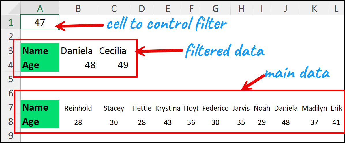
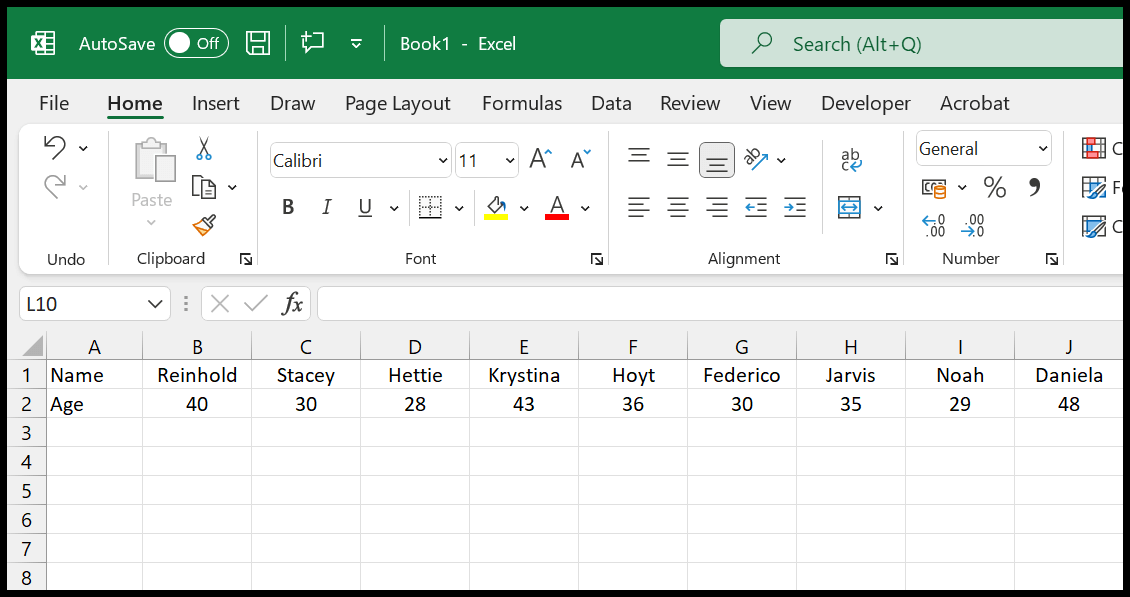
In this data, we have two rows: one row with the names and another row with the ages. The whole idea here is to filter the data based on age.
For example, if I want to filter people who are above 40 or 45, I like the filter set up so that I can enter the value in a cell, and the FILTER function will filter the data for me.
Step 1
To start with, you need to enter the filter function in cell B3, and for this, you need to type equal, the name of the function, which is filter, and then enter the starting parenthesis.
Step 2
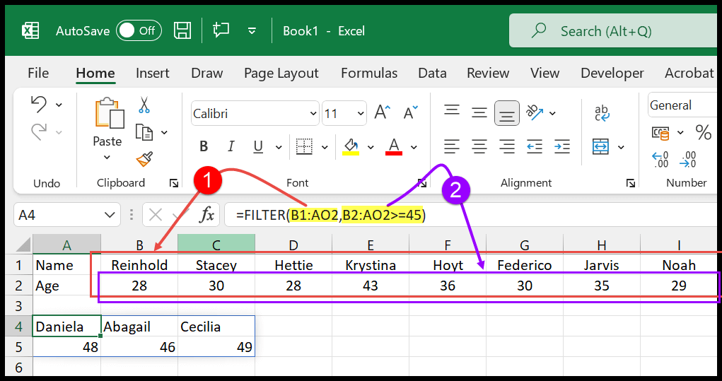
Now, in the first argument of the FILTER function, you need to specify the range or dataset arranged horizontally.
In our example, the data range is from A7 to A8, and that’s the reference you should provide in the first argument of the FILTER function.
Step 3
After that, in the second argument of the FILTER function, you need to specify the row you want to use for filtering the data. In our case, we’ll select the range A8 to AO8, which contains the age values.
Step 4
Next, along with the criteria range, we also need to specify the criteria itself. In this case, we want to filter the data where the age is greater than or equal to 45.
So, we’ll use the greater than or equal sign (>=) followed by 45 as the condition to filter the data horizontally.

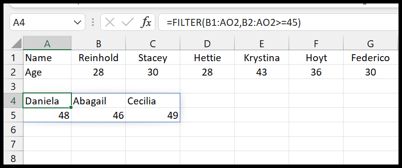
As you can see, we have filtered data from the original data that we have in the horizontal form.
=FILTER(B1:AO2,B2:AO2>=45)How Does this Formula Work?
Before we try to understand this formula, we need to know that FILTER is a DYNAMIC ARRAY FUNCTION that allows you to work with multiple values at the same time in a single formula and then return values in multiple cells.
Now, let’s split this function into two parts to understand this:
In the first part, we have referred to the entire range where we have name and age, which is B1:AO2. When you refer to this, it tells Excel to take two different arrays, as we have rows A and B.
Now, in the second part, we have referred only to the age column, and along with that, we have specified a condition to test, which is equal to or greater than 45.
Now the entire magic of this function is in this part. When specifying a condition to filter, it tests each value in the age column.
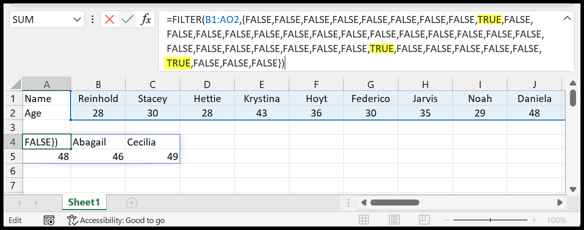
On testing, it founds only three values that are greater than or equal to 45 in the age column. This tells the FILTER function that there are three values we need to filter.
As I said, it’s a dynamic function; when selecting any of the cells, the entire filtered data is highlighted.
You can also go one step ahead and transpose data and filter horizontal data, and transpose it into vertical data by using the transpose function.
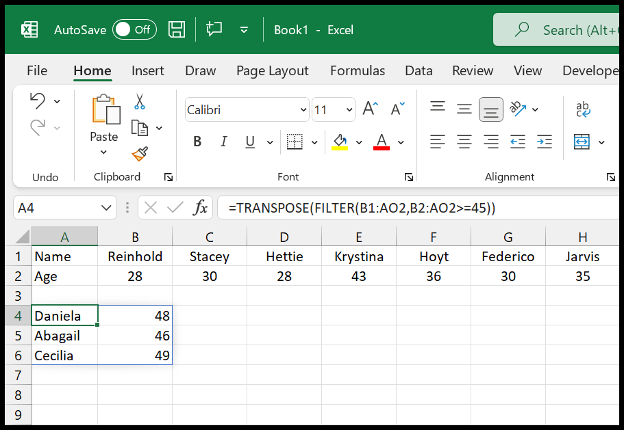
You need to wrap the filter function in the transpose function.