Pivot Tables are one of the Intermediate Excel Skills, and this is an Advanced Pivot Table Tutorial that helps you to master pivot tables.
The fact is that when it comes to data analysis, quick and effective reporting, or presenting summarized data, nothing can beat a pivot table.
It is dynamic and flexible. Even if you compare formulas and pivot tables, you will find that pivot tables are easy to use and manage. If you want to take your pivot table skills to the best, the best way is to have a list of tips and tricks that you can learn.
In this tutorial, I’ve used the words “Analyze Tab” and “Design Tab”. To get both of these tabs on the Excel ribbon, you need to select a pivot table first. Apart from this, make sure to download this sample file from here.
Tips and Tricks to Help You Become a Pivot Table PRO
1. Recommended Pivot Tables
There is an option in the “Insert Tab” to check for the recommended pivot tables. When you click on the “Recommended Pivot Tables”, it shows you a set of pivot tables that can be possible with the data you have.

This option is quite useful when you want to see all the possibilities you have with the available data.
2. Creating a Pivot Table from Quick Analysis
There is a tool in Excel called “Quick Analysis” which is like a quick toolbar that appears whenever you select the data range.
From this tool, you can create a pivot table as well. Quick Analysis Tool ➜ Tables ➜ Blank Pivot Table.

3. External Workbook as a Source for the Pivot Table
This is one of the most useful pivot table tips from this list which I want you to start using from now onward.
Let’s say, you want to create a pivot from a workbook that is in a different folder, and you don’t want to add data from that workbook into your current sheet. You can link that file as a source without adding data into the current file, here are the steps.
- In the create pivot table dialog box, select “Use an external data source”.

- After that, go to the Connections tab and click on “Browse for more”.

- Locate the file that you want to use and select it.
- Click OK.
- Now select the sheet in which you have data.

- Click OK (Twice).

Now you can create a pivot table with all the field options from the external source file.
4. The Classic Pivot Table and Pivot Chart Wizard
Instead of creating a pivot table from the Insert tab, you can use “Classic Pivot Table and Pivot Chart Wizard” as well.
The one thing I love about Classic Wizard is there is an option to pull data from multiple worksheets before creating a pivot table.
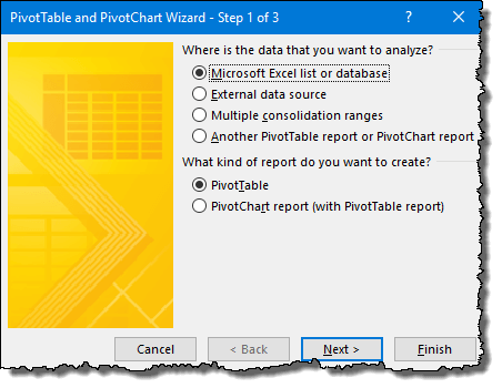
A simple way to open this wizard is by using the keyboard shortcut: Alt + D + P.
5. Search for Fields
In the pivot table field settings, there is an option for searching for the fields. You can search for the field where you have a large with hundreds of columns.

When you start typing in the search box it starts filtering columns.
6. Change Pivot Table Field Window Style
There is an option that you can use to change the style of the “Pivot table Field Window”. Click on the gear icon on the top right side and select the style you want to apply.

7. Sort the Order of your Field List
If you have a large data set then you can sort the field list using A to Z order to make it easy for you to find the required fields.
Click on the gear icon on the top right side and select “Sort A to Z”. By default, fields are sorted as per source data.

8. Open/Show Field List
It happens to me that when I create a pivot table and again when I click on it shows “Field List” on the right side and this happens every time I click on a pivot table.
But you can turn it OFF and for this, you just need to click on the “Feild List Button” in the “PivotTable Analyze” tab.

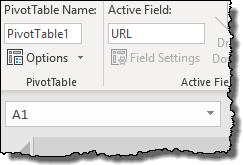
9. Naming a Pivot Table
Once you create a pivot table the next thing which I think you need to do is to name a pivot table.
For this, you can go to Analyze Tab ➜ Pivot Table ➜ Pivot Table Options and then enter the new name.
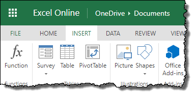
10. Create a Pivot Table in Excel Online Version
Recently, the option to create a pivot table has been added to Excel’s online App (Limited Options).
It’s as simple as creating a pivot in Excel’s Web App:
In the Insert Tab, click on the “Pivot Table” button from the table group…
…and then select the source data range…

…and the worksheet where you want to insert it…
…and, in the end, click OK.
11. Changing the Pivot Table Style or Creating a New Style
There are several pre-defined styles in Excel for a pivot table that you can apply with a single click.
In the designed tab, you can find “Pivot Table Style” and when you click on the “More” you can simply select a style which you like.
You can also create a new style, a customized one, you can do this by using the “New PivotTable Style” option.

Once you have done with your customized style you can simply save it to use it next time, it will be there always.
12. Preserve Cell Formatting when you Update a Pivot Table
Go to the pivot table options (right-click on the pivot table and go to pivot table options) and tick mark the “Preserve cell formatting on update”.
The benefit of this option is whenever you update your pivot table you won’t lose the formatting you have.
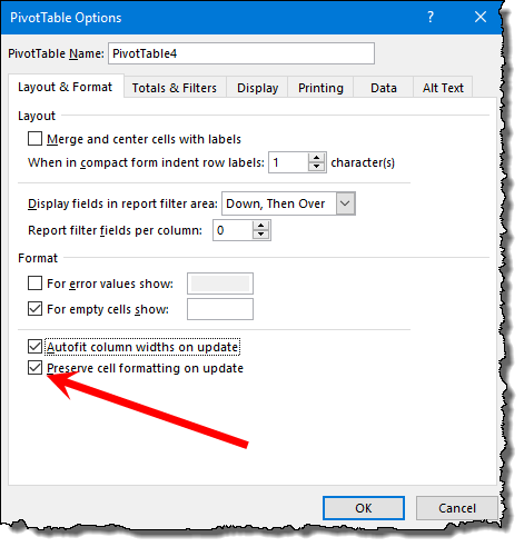
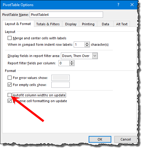
13. Disable Auto Width Update when you Update a Pivot Table
Apart from formatting one which you also need to preserve and that’s “Column Width”. For this, go to “Pivot Table Options” and untick the “Autofit column width on update” and click OK after that.
14. Repeat Item Labels
When you use more than one item in a pivot table you can simply repeat labels for the top items. It makes it easy to understand the structure of the pivot table.
- Select the pivot table and go to the “Design tab”.
- In the design tab, go to Layout ➜ Report Layout ➜ Repeat All Item Labels.

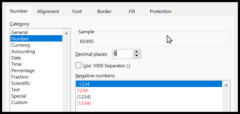
15. Formatting Values
In most of the cases, you need to format values after you create a pivot table.
For example, if you want to change the number of decimals from the numbers. All you need to do is select the values column and open the “Format Cell” option.
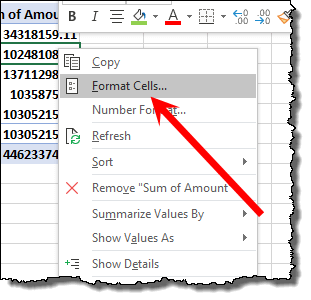
From this option, you can change the number of decimals. From the “Format” option, you can even change other
16. Change Font Style for Pivot Tables
One of my favorite things with formatting is changing “Font Style” for a pivot table. You can use the format option, but the easiest way is to do it from the Home Tab. Select the entire pivot table and then select the font style.

17. Hide/Unhide Subtotals
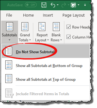
When you add a pivot table with more than one item field you will get subtotals for the main field. But sometimes there is no need to show subtotals. In that situation, you can hide them using the following steps:
- Click on the pivot table and go to the Analyze tab.
- In the Analyze tab, go to Layout ➜ Subtotals ➜ Do not show subtotals.
18. Hide/Unhide Grand Total
Just like subtotals you can also hide and unhide grand totals and below are the simple steps to do that.
- Click on the pivot table and go to the Analyze tab.
- In the Analyze tab, go to Layout ➜ Grand Total ➜ Off for Rows and Columns.

19. Two Number format in a Pivot Table
In a normal pivot table, we have a single format of values in the values column.
But, there are some (few) situations when you need to have different formats in a single pivot table, just like below. For this, you need to use custom formatting.
20. Applying a Theme to Pivot Table
In Excel, there are predefined colour themes that you can use. These themes can be applied to pivot tables as well. Go to the “Page Layout” tab, and click on the “Themes” dropdown.

There are more than 32 themes that you can apply with a single click or you can save your current formatting style as a theme.
21. Changing the Layout of a Pivot Table
For every pivot table, you can choose a layout.
In Excel (if you are using 2007 or greater versions) you can have three different layouts. In the design tab, go to the Layout Report ➜ Layout, and select the layout which you want to apply.

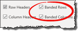
22. Banded Columns and Rows
One of the first things that I do when I create a pivot table is apply “Branded Row and Column”.
You can apply it from the design tab and tick mark the “Banded Column” and “Banded Rows”.
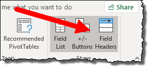
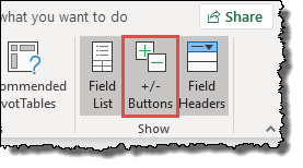
23. Turn Off/On Filters
Just like a normal filter, you can turn on/off filters in a pivot table. In the “Analyze Tab”, you can click the “Field Header” button to turn it On or OFF the filters.
24. Current Selection to the Filter
You have selected a cell(s) in a pivot table and you want to filter only those cells, here’s the option that you can use.
After selecting the cells right click and go to “Filter” and after that select “Keep Only Selected Items”.

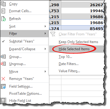
25. Hide Selection
Just like filtering the selected cells, you can also hide them. For this, go to “Filter” and after that select “Hide Selected Items”.
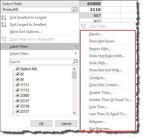
26. Value and Label Filter
Apart from normal filters, you use label filters and values filters to filter with a specific value or criteria.
Label Filter:
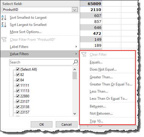
Value Filter:
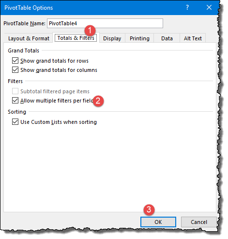
27. Use Label & Value Filter Together
As I said in the above tip that you can have the Label and Value field, but, you need to activate an option to use both of these filter options altogether.
- First of all, open the “PivotTable options” and go to the “Total & Filter” tab.
- In the “Total & Filter” Tab, tick mark the “Allow multiple filters per field”.
- After that, click OK.
28. Filter Top 10 Values
One of my favourite options in filters is to filter “Top 10 Values”. This filter option is useful while creating an instant report.
For this, you need to go to the “Value Filter” and click on the “Top 10” and then click OK.

29. Filter Fields from the PivotTable Fields Window
If you want to filter while creating a pivot table, you can do this from the “Pivot Field” window.
To filter values from a column, you can click on the down arrow from the right side and filter the values as you need.

30. Add a Slicer
One of the best things which I have found to filter data in a pivot table is using a “Slicer”.
To insert a slicer all you need to do is go to “Analyze Tab” and in the “Filter” group click on the “Insert Slicer” button, after that select the field for which you want to insert a slicer and then click OK.

Related: Excel SLICER – A Complete Guide on how to Filter Data with it
31. Format a Slicer and Other Options
Once you insert a slicer you can change its style and format.
- Select the slicer and go to the Options tab.
- From the “Slicer Styles” click on the drop-down and select the style you want to apply.

Apart from the styles, you can change the settings from the settings window: Click on the “Slicer Settings” button to open the settings window.

32. Single Slicer for all the Pivot Tables
Sometimes when you have multiple pivot tables, it’s hard to control all of them. But if you connect a single slicer with multiple pivot tables, you can control all the pivots with no effort.
- First of all, insert a slicer.
- And, after that, right-click on the slicer and select “Report Connections”.
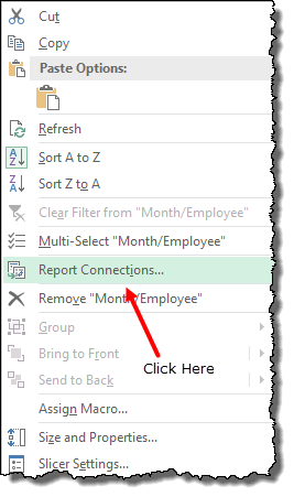
- From the dialog box, select all the pivots and click OK.
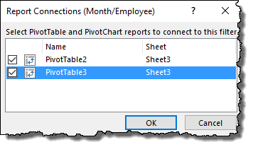
Now you can simply filter all the pivot tables with a single slicer.
33. Add a Timeline
Unlike a slicer, a timeline is a specific filter tool to filter dates and it’s way more powerful than the normal filter.
To insert a slicer all you need to do is go to “Analyze Tab” and in the “Filter” group click on the “Insert Timeline” button and after that select the date column and click OK.

34. Format a Timeline Filter and Other Options
Once you insert a timeline you can change its style and format.
- Select the timeline and go to the Options tab.
- From “Timeline Styles” click on the drop-down and select the style you want to apply.

Apart from the styles, you can change settings as well.

35. Filter using Wildcards
You can use Excel Wildcard Characters in all the filter options where you need to enter the value to filter. Look at the below examples where I have used an asterisk to filter values starting letter A.

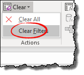
36. Clear All Filters
If you have applied filters on multiple fields, you can remove all those filters from Analyze Tab ➜ Actions ➜ Clear ➜ Clear Filter.
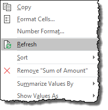
37. Refresh a Pivot Table Manually
Pivot tables are dynamic, so when you add new data or update values into the source data you need to refresh it so that the pivot table gets all the new add values from the source. Refreshing a pivot table is simple:
- One, right-click on a pivot and select “Refresh”.
- Second, go to the “Analyze” tab and click on the “Refresh” button.
38. Refresh a Pivot Table while Opening a File
There’s a simple option in Excel which you can activate and make a pivot table get refreshed automatically every time you open the workbook. For this here are the simple steps:
- First of all, right-click on a pivot table and go to “Pivot Table Options”.
- After that, go to the “Data” tab and tick mark the “Refresh the data when opening the file”.

- In the end, click OK.
Now every time you open the workbook this pivot table will get updated instantly.
39. Refresh Data After a Specific Time Interval
If you want to update your pivot table automatically after a specific interval then this tip is for you.
…here’s how to do it.
- First of all, while creating a pivot table, in the “Create Pivot Table” window, tick mark “Add this data to the data model”.

- After that, once you create a pivot table, select any of the cells, and go to the “Analyze Tab”.
- In Analyze Tab, Data ➜ Change Data Source ➜ Connection Properties.
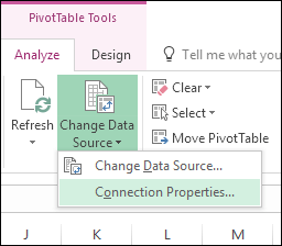
- Now in “Connection Properties”, in the usage tab, tick mark “Refresh Every” and enter minutes.

- In the end, click OK.
Now after that specific period which you entered your pivot will automatically be refreshed.
40. Replace Error Values
Sometimes, when you have errors in your source data they reflect in the same way in the pivot and this is not a good thing at all.
The better way is to replace those errors with a meaningful value. Below are the steps to follow:
- First of all, right-click on your pivot table and open the pivot table options.
- Now in “Layout & Format”, tick the mark “For error value show” and enter the value in the input box.

- In the end, click OK.
Now for all the errors, you will have the value you have specified.
41. Replace Blank Cells
Let’s say you have a pivot for sales data and there are some cells that are blank.
For a person who is not aware of why these cells are blank can question you about this. So, it’s better to replace it with a meaningful word.
…simple steps you need to follow for this.
- First of all, “right click” on your pivot table and open pivot table options.
- Now in “Layout & Format”, tick mark “For empty cells show” and enter the value in the input box.
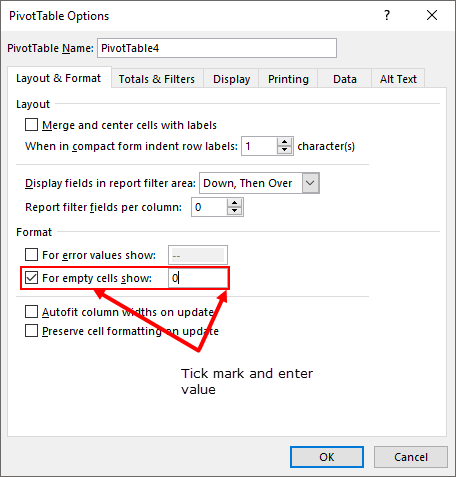
- In the end, click OK.
Now for all the blank cells, you will have the value you have specified.
42. Define a Number Format
Let’s say you have a pivot for sales data and there are some cells that are blank.
For a person who is not aware of why these cells are blank can question you about this. So, it’s better to replace it with a meaningful word.
…simple steps you need to follow for this.
- First of all, “right click” on your pivot table and open pivot table options.
- Now in “Layout & Format”, tick mark “For empty cells show” and enter the value in the input box.
- In the end, click OK.
Now for all the blank cells, you will have the value you have specified.
43. Add a Blank Row after Each Item
Now let’s say you have a large pivot table with multiple items.
Here you can insert a blank row after each item so that there would be no clutter in the pivot.

Check out these steps to follow:
- Select the pivot table and go to the Design tab.
- In the design tab, go to Layout ➜ Blank Rows ➜ Insert Blank Line after Each Item.

The best thing about this option is it gives a clearer view of your report.
44. Drag and Drop Items in a Pivot Table
When you have a long list of items in your pivot you can arrange all those items in a custom order by just drag and drop.
45. Creating many Pivot Tables from One
Suppose you have created a pivot table from month-wise sales data and you have used products as a report filter.
With the”Show Report Filter Pages” option, you can create multiple worksheets with a pivot table for each product.
Let’s say if you have 10 products in a pivot filter you can create 10 different worksheets with a single click.
Use these steps:
- Select your pivot and go to the analyze tab.
- In the analyze tab, go to pivot table ➜ Options ➜ Show Report Filter Pages.

Now you have four pivot tables in four separate worksheets.

46. Value Calculation Option
When you add a value column into the value field it shows SUM or COUNT (sometimes), but, there few other things which you can calculate here:
To open the “Value Settings” options select a cell from the value column and right-click.
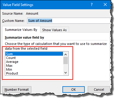
And from the right-click menu, open “Value Field Settings” and then click on
From the “Summarize value field” select the type of calculation which you want to show in the pivot.
47. Running Total Column in a Pivot Table
Let’s say you have a pivot table month-wise sale.
Now, you want to insert a running total in your pivot table to show a complete growth of sales in the entire month.
Here are the steps:
- Right-click on it & click “Value Field Setting”.
- From the “Show Values As” drop-down list, select “Running Total In”.

- In the end, click OK.

48. Add Ranks in a Pivot Table
The ranking gives you a better way to compare things with each other…
…and to insert a rank column in a pivot table you can use the following steps:
- First of all, insert the same data field twice in the pivot.
- After that for the second field, right-click on it and open “Value Field Settings”.
- Go to the “Show Values as” tab and select “Rank Largest To Smallest”.

- In the end, click OK.
Imagine you have a pivot table for product-wise sales. And now, you want to calculate the percentage share of all products in the total sales. Steps to use:
- First of all, insert the same data field twice in the pivot.
- After that for the second field, right-click on it and open “Value Field Settings”.
- Go to “Show Values as” tab and select “% of Grand Total”.

- In the end, click OK.

This is also a perfect option to create a quick report.
50. Move a Pivot table to a New Worksheet
When you create a pivot table, Excel asks you to add a new worksheet for the pivot table, but it also has an option to move an existing pivot table to a new worksheet.
- For this, go to “Analyze Tab” ➜ Actions ➜ Move Pivot Tables.

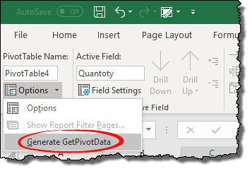
51. Turn OFF GetPivotData
There is a situation where you need to refer to a cell in a pivot.
However, there could be a problem because when you refer to a cell in a pivot Excel automatically uses the GetPivotData function for reference. The best thing is, that you can disable it and here are the steps:
- Go to File Tab ➜ Options.
- In options, go to Formulas ➜ Working with Formulas ➜ untick “Use GetPivotData functions for PivotTable reference”.
You can also use a VBA code for this as well:
Sub deactivateGetPivotData()
Application.GenerateGetPivotData = False
End Sub
52. Group Dates in a Pivot Table
Just imagine, you want to create a month-wise pivot table but you have dates in your data. In this situation, you need to add an extra column for months.
But the best way is to create using grouping dates methods in the pivot table using this method you don’t need to add a helper column. Use the below steps:
- First of all, you need to insert the date as a row item in your pivot table.

- Right click on the pivot table, and select “Group…”.

- Select “Month” from by section and click OK.
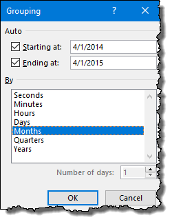
It will group all the dates into months and if you want to learn more about this option here’s the complete guide.
53. Group Numeric Data in a Pivot Table
Just like dates, you can group numeric values as well.
The steps are simple.
- Right-click on the pivot table, and select “Group…”.
- Enter the value to create a range of groups in the “by” and click OK.
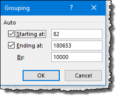
…click here to learn how the pivot table’s grouping option can help you create a histogram in Excel.
54. Groups Columns
To group columns just like rows, you can use the same steps as rows. But you need to select a column header before that.
55. Ungroup Rows and Columns
When you don’t need groups in your pivot table you can simply ungroup it by right-clicking and selecting “Ungroup”.
56. Using Calculation in a Pivot Table
To become an advanced pivot table user you should learn to create a calculated field and item in a pivot table.
Let’s say in the below pivot table, you need to create new data by field multiplying the present data field with 10.
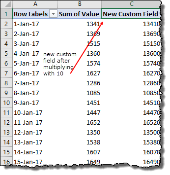
In this situation, instead of creating a separate column in a pivot table, you can insert a calculated item.
➜ a complete guide to creating a calculated item and field in a pivot table
57. List of Formulas Used
Once you add a calculation in a pivot table or you have a pivot table with a calculated field or item, you can see the list of formulas used in it.
For this, just go to “Analyze Tab” ➜ Calculation ➜ Fields, Items & Sets ➜ List Formulas.
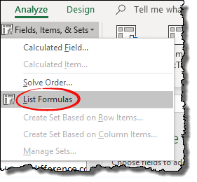
You’ll instantly get a new worksheet with a list of formulas used in the pivot table.
58. Get a List of Unique Values
If you have duplicate values in your date, you can use a pivot table to get a list of unique values.
- First, you need to insert a pivot table and then add the column with duplicate values as a row field.
- After that, copy that row field from the pivot and paste it as values.
- Now, the list you have as values is a list of unique values.
The thing which I love about using a pivot table to check unique values is it’s a one-time setup.
You don’t need to create it again and again.
59. Show Items with No Data
Let’s say you have entries in your source data where there are no values or zero values.
You can activate from the field option to “Show items with no data”.
- First of all, right-click on the field and open the “Field Settings”.
- Now, go to “Layout & Print” and tick mark “Show items with no data” and click OK.

Boom! All the items where you have no data will show in the pivot table.
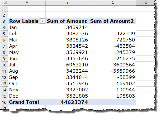
60. Difference from the Previous Value
This is one of my favorite pivot table options. With this, you can create a column that shows the difference of current values from the previous value.
Let’s say you have a pivot with month values, then, with this option you can add a column of difference value from the previous month, just like below.
Here are the steps:
- First of all, you need to add the column where you have values, twice in the value field.

- After that, for the second field, open the “Value Setting” and “Show Value As”.
- Now, from the “Show values as” drop-down select “Difference From” and select “Month” and “(Previous)” from the “Base Item”.
- In the end, click OK.

This will instantly convert the values column into a column with a difference from the previous.
61. Disable Show Details
When you double-click on a value cell in a pivot table it shows the data behind that value.
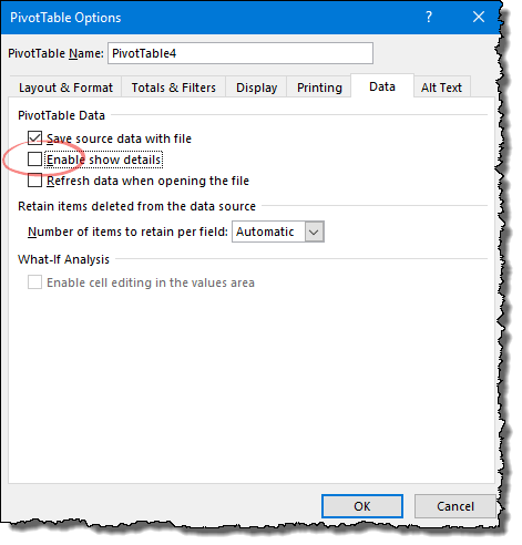
It’s a good thing but not all the time you need this to happen and that’s why you can disable it when required. All you need to do is open the pivot table options, go to “Data Tab” and untick “Enable show details”.
And then click OK.
62. Pivot Table to PowerPoint
These are the simple steps to paste a pivot chart into a PowerPoint slide.
- First of all, select a pivot table and copy it.
- After that, go to the PowerPoint slide and open the Paste special options.

- Now from the paste special dialog box, select “Microsoft Excel Chart Object” and click OK.
Insert Image
To make changes to the pivot table you need to double click on the chart.
63. Add Pivot Table to Word Document
To add a pivot table into Microsoft Word you need to follow the same steps you did in PowerPoint.
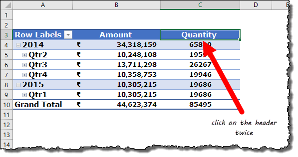
64. Expand or Collapse Field Headings
If you have more than one dimension field in a row or column you can expand or collapse the outer fields. You need to click on the + button to expand and the – button to collapse…

…and to expand or collapse all the groups in one go, you can right-click and choose the option.
65. Hide-Unhide Expand or Collapse Buttons
If you have more than one dimension field in a row or column you can expand or collapse the outer fields.
66. Only Count Numbers in Values
There is an option in a pivot table where you can count the number of the cell with the numeric value.

For this, all you need to do is open the “Value Option” and select “Count Number” from the “Summary value field by” and then click OK.
67. Sort Items According to a Corresponding Value
Yes, you can sort according to the corresponding values.
- All you need to do is open the filter and select the “More Sort Option”.
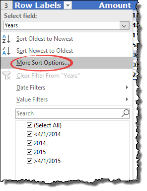
- Then select “Accessing (A to Z) by:” and select the column for sorting and then click OK.

Note: If you have multiple value columns, you can only use one column for sorting order.
68. Custom Sort Order
Yes, you can use a custom sorting order for your pivot table.
- For this, when you open “More Sorting Options”, click on “More Options” and untick the “Sort automatically every time the report is updated”.
- After that select the sorting order and click OK in the end.
You need to create a new custom sorting order then you can create it from File Tab ➜ Options ➜ Advanced ➜ General ➜ Edit Custom List.
69. Deferred Layout
If you enable the “Deferred Layout Update” and drag and move fields between areas after that.
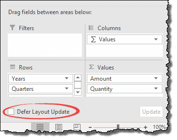
Your pivot table will not update unless you click on the Update button below at the corner of the PivotTable Fields. It makes it easier for you to check the pivot table and then.
70. Changing Field Name
When you insert a value field, the name you get for the field comes something like this “Sum of the Amount” or “Count of Units”.
But sometimes (well, all the time) you need to change this name to the name without “Sum of” or “Count of”.
For this, all you need to do is to remove “Count of” or “Sum of” from the cell and add a space at the end of the name. Yes, that’s it.
71. Select the Entire Pivot Table
If you want to select an entire pivot table in one go: Select any of the cells from the pivot table and use the keyboard shortcut Control + A. Or go to the Analyze tab ➜ Select ➜ Entire Pivot Table.

72. Convert to Values
If you want to convert a pivot table in values, all you need to do is select the entire pivot table and then: Use Control + C to copy it and then Paste Special ➜ Values.
73. Use Pivot Table in a Protected Worksheet
When you’re protecting a worksheet where you have a pivot table, make sure to tick mark:
“Use PivotTable & PivotChart”
from the “Allow all the users of this worksheet to:”.
74. Double Click to Open Value Field Settings
If you want to open the “Value Settings” for a particular value column…
…then…
…the best way is to double-click on the header of the column.
75. Reduces the Size of a Pivot Table Report
If you think like this: when you create a pivot table from scratch, Excel creates a pivot cache.
So, the more pivot tables you create from scratch more pivot cache Excel will create and your file will need to store more data.
So, what’s the point? Make sure all pivot tables which are from data sources must have the same cache.
But Puneet how could I do this? Simple, whenever you need to create a second, third, or fourth. Just copy and paste the first one and make changes to it.
76. Delete the Source Data and the Pivot Table still Works Fine
One more thing which you can do before sending a pivot table to someone is delete the source data. Your pivot table will still work fine. And, if someone needs to have the source data can get it by clicking the grand total of the pivot table.
77. Save a Pivot Table as a Web Page [HTML]
One more way you can use to share a pivot table with someone is to create a webpage. Yes, a simple HTML file with a pivot table.
- For this, all you need to do is to save the workbook as a web page [html].
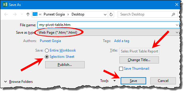
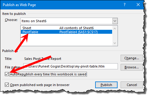
- In the Publish as Web Page, select the pivot table and click “Publish”.
Now you can send this HTML web page to anyone and he/she can view the pivot table (not editable) even on their mobile phone.

78. Save a Pivot Table as a Web Page [HTML]
One more way you can use to share a pivot table with someone is to create a webpage. Yes, a simple HTML file with a pivot table.
- For this, all you need to do is to save the workbook as a web page [html].
- In the Publish as Web Page, select the pivot table and click “Publish”.
Now you can send this HTML web page to anyone and he/she can view the pivot table (not editable) even on their mobile phone.
79. Creating a Pivot Table Through a Workbook from a Web Address
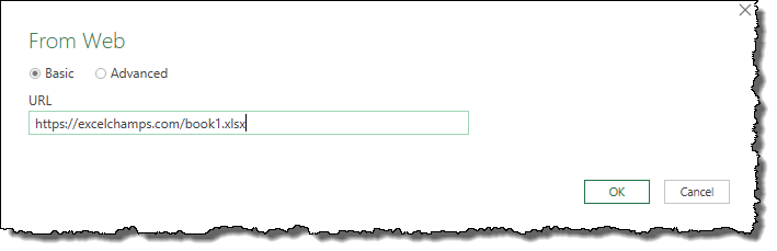
Let’s say you have a web link for an Excel file, just like the one below:
https://excelchamps.com/book1.xlsx
In this workbook, you have the data and with that data, you need to create a pivot table. For this, the POWER QUERY is the key.
Check this out: Power Query Examples + Tips and Tricks
- First of all, go to the Data Tab ➜ Get & Transform Data ➜ From Web.
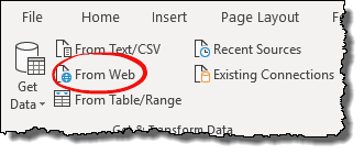
- Now, in the “From Web” dialog box, enter the web address of the workbook and click OK.
- After that, select the worksheet and click “Load To”.

- Next, select the PivotTable Report and click OK.

At this point, you have a blank pivot table that is connected to the workbook from the web address you have entered.
Now you can create a pivot table as you want.
80. Applying General CF Options
There are all the CF options available to use with a pivot table.
➜ here is the guide which can help you learn all the different ways to use CF in pivot tables.
81. Highlight Top 10 Values
Instead of filtering, you can highlight the top 10 values from a pivot table. For this, you need to use conditional formatting.
The steps are below:
- Select any of the cells from the value column from your pivot table.
- Go to Home tab ➜ Styles ➜ Conditional Formatting.
- Now in conditional formatting, go to Top/Bottom Rules ➜ Top 10 Items.

- Select the colour from the window you have.
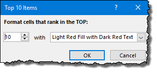
- And in the end, click OK.
This option is quite useful while creating quick reports with a pivot table and once you.
82. Remove CF from a Pivot Table
You can simply remove conditional formatting from a pivot table using the below steps:
- First of all, select any of the cells from the pivot table.
- After that, go to Home Tab ➜ Styles ➜ Conditional Formatting ➜ Clear Rules ➜ “Clear rules from This Pivot Table”.

If you have more than one pivot table then you need to remove CF one by one.
Before you create a pivot table, spend a few minutes reviewing the data source to check if any corrections are needed.
No Blank Column and Row in the Source Data
One of the things you need to keep in check in the source data is that there shouldn’t be any blank rows or columns. When creating a pivot table, if you have a blank row or column, Excel will only include data up to that row or column.

No Blank Cell in the Value Column
Apart from the blank row and column, you must not have a blank cell in the column where you have values.

The biggest reason to keep a check on this is that if you have a blank cell in the values field column: Excel will apply count in the pivot instead of the SUM of the values.
Data should be in the Right Format
When you are using source data for a pivot table then it must be in the right format. Let’s suppose, you have dates in a column and that column is formatted as text. In that case, it wouldn’t be possible to group dates in the pivot table that you have created.

Use a Table for Source Data
Before you create a pivot table, you should convert your source data into a table.

A table expands itself whenever you add new data to it and it makes changing the pivot table data source easy (almost automatic). Here are the steps:
- Select your entire data or any of the cells.
- Press the shortcut key Ctrl + T.
- Click OK.
Remove Totals from the Data
Last but not least, ensure that you delete the total from the data source.

If you have source data with grand totals, Excel will use those totals as values, and the values in the pivot table will be doubled.
Tip: If you have applied a table on the data source, Excel won’t include that total while creating a pivot table.
You can download this data from here to create your first pivot table in Excel. Make sure to learn some of the tips that can help you get the data before creating a pivot.
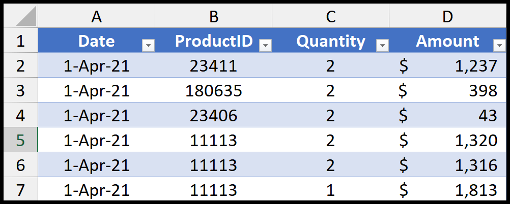
Now, this data has four columns, and you need a year- and month-wise pivot table to analyze data.
- First, go to the Insert Tab > Tables > Pivot Table > From Table/Range. Or you can also use the keyboard shortcut Alt > N > V > T.

- It will open the “PivotTable from table or Range” dialog box to select the range or table. When you open the dialog box, it automatically selects the range or the table.
- You can select the worksheet in the same dialog box to insert the pivot table. You can select the same worksheet where you have the data or a new worksheet.

- Next, click the OK button to insert the pivot table into a new sheet. When you click OK, it instantly inserts a new sheet and creates a blank pivot table. And once you do this, you need to create a pivot table.

- Insert columns, rows, values, and filters on the right side of the PivotTable pane. Here, we need to create a pivot table month-wise, so you must drag and drop the date column to the rows.
- When you enter the date column into the rows, Excel automatically splits the date into three more parts: year, quarter, and months. You can see in the below snapshot that we have three more columns that are extracted from the original date column along with the date.

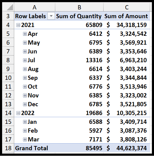
- In the pivot table, you can see a structure where you have years, quarters, months, and then further dates.

- As you don’t need quarters, please remove it from the rows box from the right-side pane. It will also remove the quarters from the pivot table instantly.

- The next thing is to add the values column to the values field. For this, you must ensure that the column(s) you want to add to the values field must have numeric values; otherwise, it won’t show them.
- You must add the quantity and amount columns to the values field. You can see in the below snapshot that when you enter both columns into the values field.

Your pivot table is ready now.
The last thing that you need to do is to change the formatting of the values column. So, for this, select the Amount column and use the keyboard shortcut (Ctrl + 1) to open the formatting dialog box.
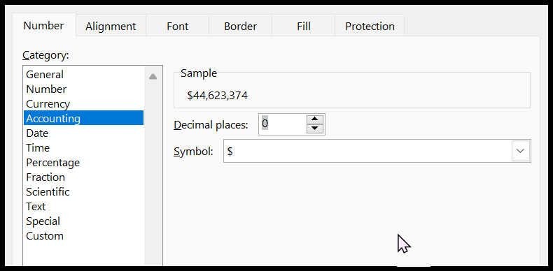
After that, select the quantity column and open the format cells dialog box; you can use the number format from there.
And here is your ready-to-present pivot table.

Using Pivot Charts with Pivot Tables to Visualize Your Report
I’m a big fan of the pivot chart. If you know how to use a pivot chart properly you can make the best out of one of the best Excel tools.
- Select a cell from the pivot table and go to “Analyze tab”.
- In the “Analyze Tab”, click on the “Pivot Chart”.
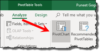
It will instantly create a pivot chart from the pivot table you have. And, when you insert a new pivot chart it comes with some buttons to filter it which sometimes are not really useful. And if you think like this, you can hide all of them or some of them.
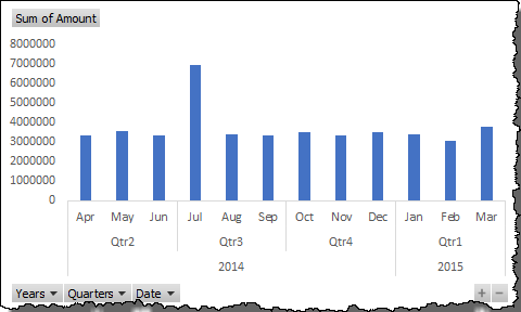
Right-click on the button and select “Hide value Field Button on the Chart” to hide the selected button or click on “Hide all the field button of the Chart” to hide all the buttons.

When you hide all the buttons from a pivot chart it also hides the filter button from the bottom of the chart but, you can still filter it using the pivot table filter, slicer, or a timeline.
In the End
As I said pivot tables are one of those tools which can help you get better in creating reports and analyzing data in no time.
And with these tips and tricks, you can even save more time. If you ask me, I want you to start using at least 10 tips first and then go for the next 10 and so on.
But you need to tell me one thing now: What’s your favorite pivot table tip?
Don’t Miss to Read These
- Add-Remove Grand Total in a Pivot Table
- Add Running Total in a Pivot Table
- Automatically Update a Pivot Table
- Formulas in a Pivot Table
- Change Data Source for Pivot Table
- Count Unique Values in a Pivot Table
- Delete a Pivot Table
- Filter a Pivot Table
- Add Ranks in Pivot Table
- Conditional Formatting to a Pivot Table
Super sir tq
Hi dear friends , I appreciate your hard work in creating these useful information and hope you all the best in life and your business .
Hi Puneet, sometimes I hit the keyboard by accident when the focus is on an empty cell, and another empty cell is placed inside the cell, I need to know how to delete the inserted cell without having to copy everything into a new sheet except for the corrupted cell… any help appreciated, this has happened to me so many times.
Thank you very much, a real treasure for me
Have a nice day
Always thankful to you for the excellent tutorials and tips!
You are welcome.