

One of the best ways to quickly analyze data in Excel is to use filters, and the best way to filter data is to use SLICER, period.
Slicer makes your data filtering experience a whole lot better. It’s fast, powerful, and easy to use. That’s why it is a part of our ADVANCED EXCEL SKILLS, and today in this tutorial, we will be exploring it in detail.
What is an Excel Slicer
An Excel Slicer is a bunch of buttons that you can use to filter data from a column. Unlike a standard filter, it shows you all the available items that you can use to filter as buttons. You can connect it with a table or a pivot table and customize it the way you want (Color, Font, Buttons, etc.).
Insert Slicer with a Table in Excel
To insert a SLICER in an Excel Table, use the following steps (slicers for tables need Excel 2013 or later; for pivot tables, Excel 2010 or later).
- First of all, press CTRL+T to convert the data (DOWNLOAD) into an Excel table, or you can also go to the Insert tab and click on Table.

- After that, select any of the cells from the table and then go to → Insert Tab → Slicer (click on the slicer button).

- Once you click on the button, you get a dialog box with all the column names to select from to insert a slicer.
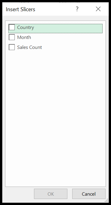
- In the end, tick the column that you want to use as a filter (you can also tick more than one column, and Excel inserts one slicer for each) and click OK.

Insert a Slicer with a Pivot Table
- Click anywhere on the pivot table.
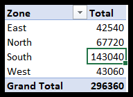
- After that, go to → Insert → Slicer (or PivotTable Analyze → Insert Slicer).

- Select the column that you want to use in the slicer. Here we have selected zone.
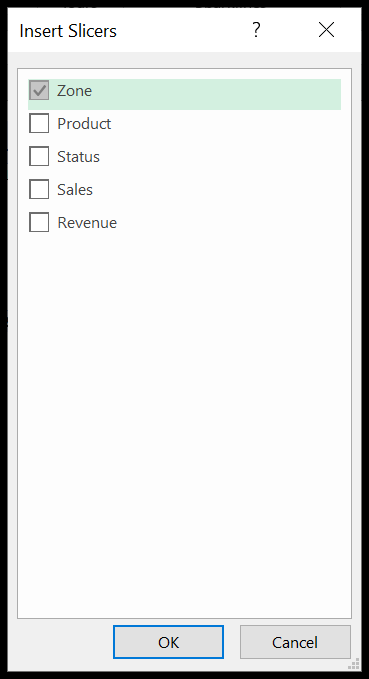
- In the end, click OK.
Related: How to Link/Connect a Single Slicer with Multiple Pivot Tables in Excel
How to use Slicer in Excel
Now we will learn how to use the Slicers since we know how to insert one. We will discuss three important things now.
1. Select a Single Slicer item
This is quite simple. As soon as you insert a slicer, you click on any button to filter your data. Let’s try to understand it with a very simple example.
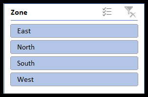
Here we have inserted a slicer of Zone. The blue highlighted buttons (East, North, South & West) are all selected. Therefore, you can see the data of all four regions in the pivot.

Now we need to filter our data for the North Zone only. Click on the North button. The data in the pivot table will automatically be filtered. As soon as you click on the North button, all the other buttons will be dimmed.

2. Select Multiple Items
Now, what if we need to select the data for two or more regions? Let’s say we need to filter the data for the East and West Zone. This is very easy. You just need to press Ctrl and click on the buttons you need to filter. You can also click the Multi-Select button on the slicer header (or press Alt + S) and then click the buttons one by one without holding Ctrl.
Like here we will press Ctrl and click on East & West.

You can also select two or more consecutive buttons by simply clicking and dragging. Here we could have used this method if we had to select the data for East & North, North & South, or South & West.
3. Clear Selected Items
The last and most important thing is removing the filters. Once you remove all the filters, all of your data will be visible and all the buttons will be highlighted. You can do this with a single click on the Clear Filter button at the top right of the slicer (or press Alt + C when the slicer is selected).
Formatting a Slicer
Since now we know how to work with slicers, let us start with formatting.
When it comes to useful presentable reports, format plays an important role. A well-organized, eye-catching, and good-looking report will attract more audiences than others. So, it is crucial to organize and format the reports and Slicers.
1. Remove Headers
Many times, we run short of space in our reports, especially when we are making a dashboard. Do not worry if your slicer takes up more space. We can cut it short in many ways, one of which is removing the headers.
Here in our example, we know that North, East, West & South are the Zones, so we don’t necessarily need the Header “Zone”. Let us remove the header and save some space.
Select the Slicer → Right-click → Slicer Settings.
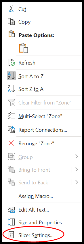
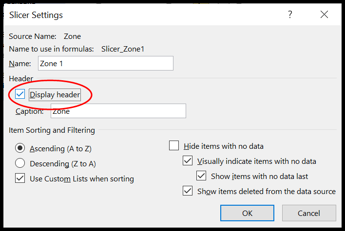
Untick the box against “Display Header”.
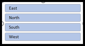
The header is removed, and we could save some space.
2. Change the Font
The next thing you need to know is how to change the font of a slicer.
- To start with, select the slicer and find the style that best suits your requirements in the Slicer Styles gallery on the Slicer tab.
- Now, right-click that style and click on Duplicate.

- Here the “Modify Slicer Style” dialog box will open, with a “Slicer Element” list.
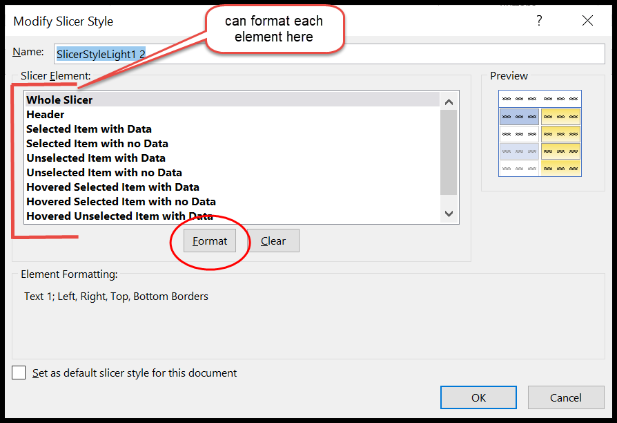
- If you closed it, right-click on the duplicate slicer style (under Custom in the gallery) and click Modify.
- Now select “Whole Slicer” in the list and click Format.
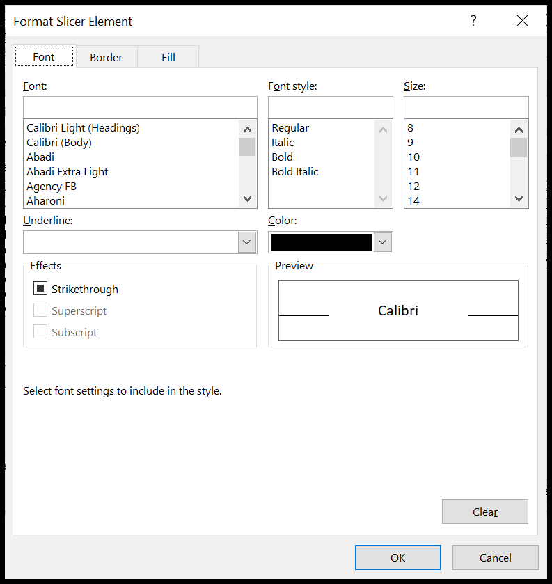
- Customize the font, borders, and fill as per your requirements.
- Apply the new style to your slicer by clicking it under Custom in the Slicer Styles gallery.
- Hit OK.
3. Remove Borders
Removing borders is as easy as changing the font. First, repeat the steps you did in changing the font.
- Select the duplicate slicer style → Modify → Format → Border.

- Since we want to remove borders, click on “None”.
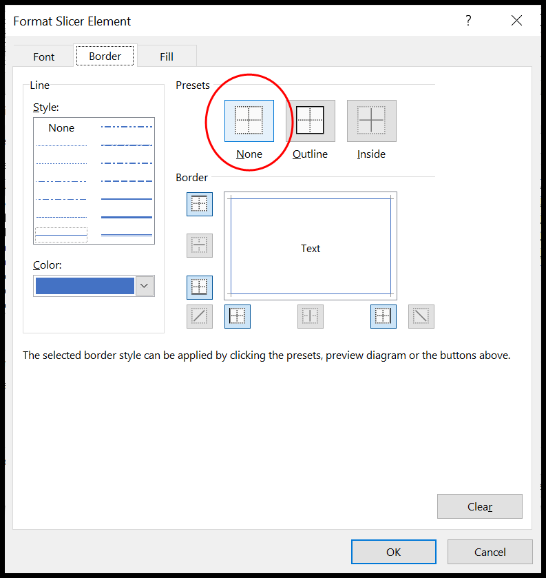
- Now hit OK.

4. Remove Items with No Data
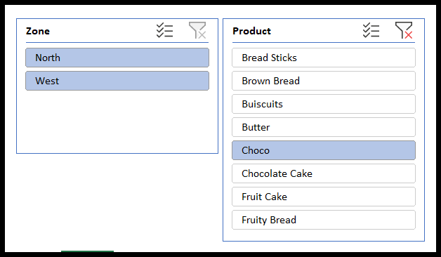
Sometimes you might find some items which are not highlighted since they do not contain any data. For example, here when I select the product “Choco”, the East and South zone buttons are not active. This means that there are no sales of “Choco” in these two zones.
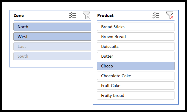
It is always advised to hide such buttons. Let us see how to do it.
- First, right-click the slicer and select Slicer settings.
- Now you will see the “Slicer settings” window.
- Tick the box against “Hide items with no data”.
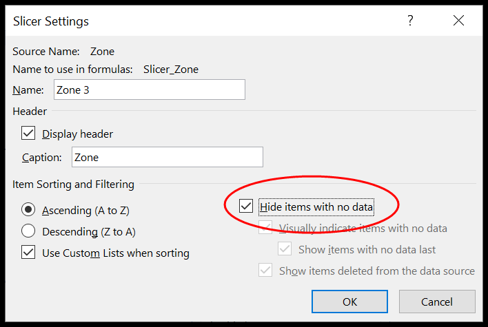
- Here we go.
5. Customize Columns and Buttons
Most of the time, the slicer may not fit into your dashboard or report due to its column-type structure. Hold on!! If this is the case, then you need to know that you can organize the distribution of the buttons in a slicer.
Select the slicer → Slicer (Top Ribbon) →Buttons
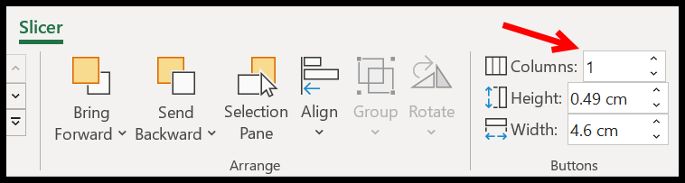
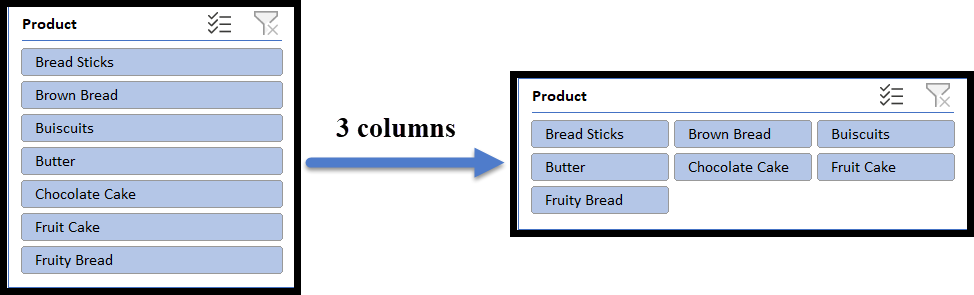
Here, increase the number of columns as per your requirement. I have increased the columns to 3, and my slicer now has three columns and is horizontally spread.
Tip: You can also adjust the height and width of the buttons from the same tab.

6. Customize Size
If you do not want to spend more time formatting the buttons or are not interested in playing with the columns and button sizes, all you need to do is adjust the dimensions of the slicer using the Size option.

You can also use the mouse, but you need good control over it. To avoid all this mess, simply select the slicer → Slicer (Top Ribbon) → Size. Here you can adjust the height and width of the Slicer as a whole. You do not need to play with each element.
7. Rename a Slicer
What if you want to rename a Slicer or put a small description in your Slicer header?

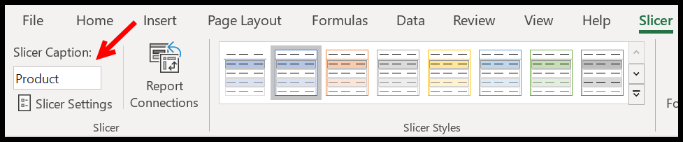
You can do this with a single click. Select the slicer → Slicer (Top Ribbon) → Slicer Caption
8. Align Slicers
The next important thing that you need to learn is alignment. When you have multiple slicers, it is always advised to align them for a better presentation. Select all the slicers → Slicer (Top Ribbon) → Arrange → Align
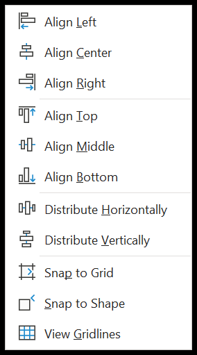
Here you have several options that are useful when you have more than one slicer (Distribute Horizontally and Distribute Vertically need at least three). Most of the time when you insert the slicers, they are cascaded over each other.
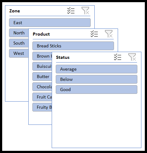
They are not distributed well. To arrange them well in your report or dashboard we have a quick fix called Align.
Align: This option helps you to line up all your slicers to the left, center, right, top, middle, or bottom. You need to decide where you want to place your slicers.
- First, select all the slicers.
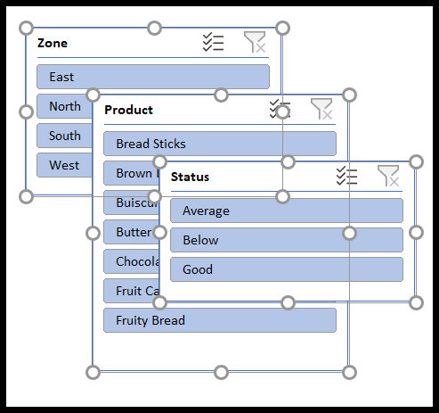
- After that click on Align Top.
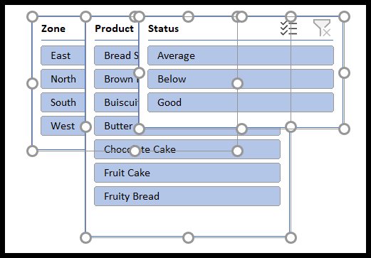
- All the slicers will have a common start point from the top.
- Now select the rightmost slicer and drag it to the right side. Here you need to think of the approximate space all your slicers will be needing.
- Here again, select all the slicers and click on distribute horizontally. Sometimes you might have to click this multiple times to adjust the spaces between the slicers.
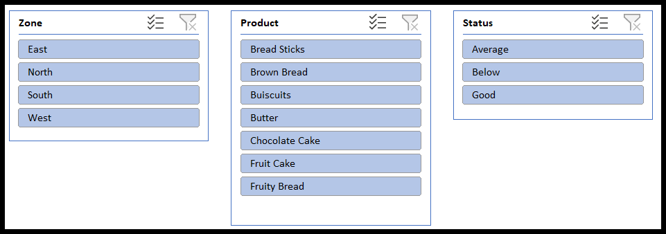
Similarly, you can distribute your slicer vertically.
Snap to Grid and Snap to Shape: In case you are running short of time and have multiple shapes In your report or dashboard, all you need to do is select all the slicers and turn on Snap to Shape (or Snap to Grid) under Arrange → Align. They are two separate options, and you can turn on one or both.
- Snap to shape helps you to adjust your shape to the other shapes in your report or dashboard.
- Snap to grid adjusts your slicer or shapes to the cell gridlines of the worksheet.
Connect One Slicer to Multiple Pivot Tables
A slicer can filter more than one pivot table at once, as long as the pivot tables use the same data source. Select the slicer, go to Slicer → Report Connections, and tick the pivot tables you want it to control. You can find all the steps in this tutorial.
Slicer vs Filter
- What you see: a slicer shows every item as a button and what’s filtered at a glance, while a filter drop-down hides the selection inside the menu.
- Conditions: a filter can do “greater than”, “contains” or date ranges; a slicer only selects items (use a Timeline for date ranges in a pivot table).
- Where it works: slicers work with Excel tables and pivot tables, not with a normal range.
Frequently Asked Questions
The active cell isn’t inside a table or a pivot table, or the workbook is in the old .xls format. Click inside the table, or save the file as .xlsx and try again.
How do I delete a slicer?
Select the slicer and press Delete. Clear its filter first (Alt + C) if you want the data to show all items again.
Can I stop users from moving a slicer?
Yes. Right-click the slicer → Size and Properties, and under Position and Layout, tick “Disable resizing and moving”.
Written by
Puneet Gogia
Microsoft MVP — Excel · Founder, Excel Champs
Twelve years of teaching Excel, and a decade before that using it as a data analyst. Every tutorial here is written from a file I actually built.