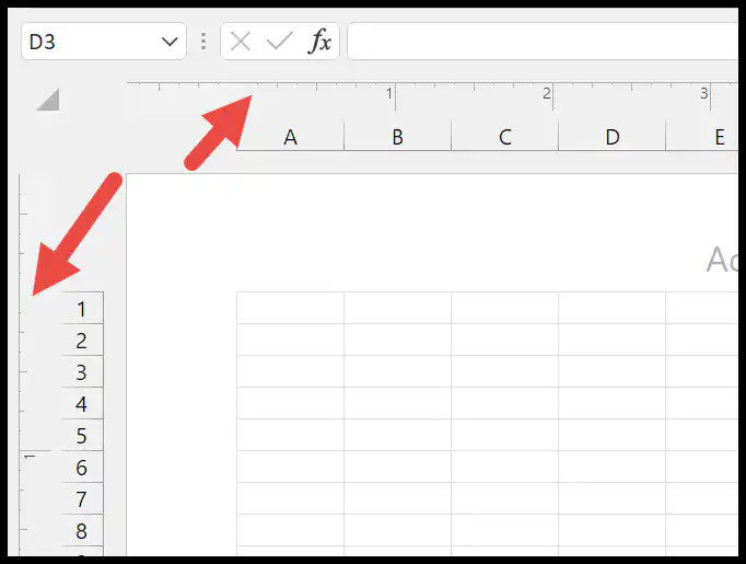
In Excel, there is an option to show a ruler around rows and columns that can help you to align the objects like charts, and images and even change column width and row height while taking a printout.
Steps to Show Ruler in Excel
- First, activate the sheet in which you want to show the ruler.
- After that, go to the View tab on the ribbon.
- From there, locate the Page Layout button in the “Workbooks View”.
- Next, click on the “Page Layout” button.
- In the end, tick-mark the “Ruler” box from the show group.
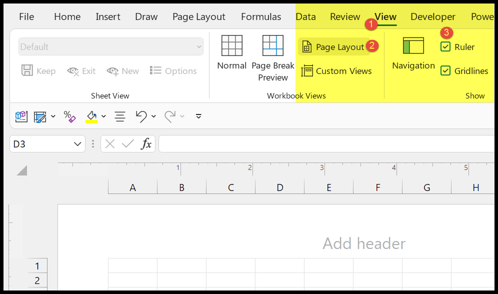
Note: The only way to show the ruler is to activate the page layout. And that’s the reason when you try to click on the ruler check box, it’s greyed out in the normal view.
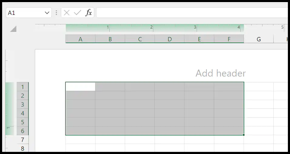
After activating the ruler, when you select a cell and range of cells, Excel highlights that part of the selection on the ruler.
Changing the Ruler Unit
When you activate the ruler, it comes with the default units that you have as per your system. But you can change the units from the Excel options.
Go to the File Tab ➟ Options ➟ Advanced. In the advanced options scroll down to the display group. In the display group, you can find the drop-down “Ruler units” to change the unit to Inches, Centimeter, or Millimeters.
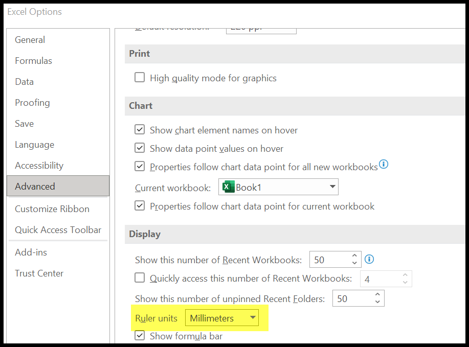
And once you choose the unit, click OK.
Note: When you change the view from normal to page layout and activate the ruler. This setting is only for the current worksheet.
Related Tutorials
- Fill Justify in Excel
- Formula Bar in Excel
- Add a Header and Footer in Excel
- Fill Handle in Excel
- Format Painter in Excel
- Quick Access Toolbar in Excel
- Status Bar in Excel
- Insert Text Box in Excel
- Keyboard’s Arrow Keys Aren’t Working in Excel (Scroll Lock ON-OFF)
- Open Backstage View in Excel
- Use Excel in Dark Mode
- Get the Scroll Bar Back in Excel