

To turn columns into rows, use =TRANSPOSE(A1:B6). In Excel 365 and 2021 you just type it into one cell and press Enter — the result spills across automatically.
On Excel 2019 and earlier you have to select the destination range first, with the dimensions reversed (six rows by two columns becomes two rows by six columns), then enter the formula with Ctrl+Shift+Enter.
The formula stays linked to the source, so editing an original cell updates the transposed copy; to break that link, copy the result and paste as values (Ctrl+Alt+V → V).
If you don’t want a live formula at all, the quicker route is to copy the range, right-click where you want it, and choose Paste Special → Transpose (Ctrl+Alt+V → E), which pastes static values in one step. And if the data is a proper table you’ll be reshaping repeatedly, Power Query’s Transpose does it as a refreshable step.
In Excel, if you want to change columns to rows, you can use the TRANSPOSE function. With this function, all you need to do is select a range with equivalent cells from where you want to add the changed data, refer to the range, and use CONTROL + SHIFT + ENTER.
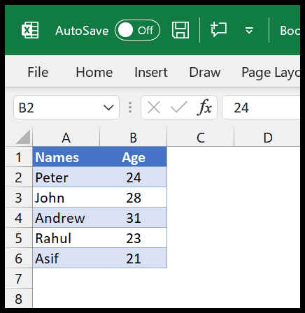
In the following example, you have a list of names and ages. And we need to change these two columns into rows.

Steps to Change Columns to Rows
- First, in the range D1:H2, enter the TRANSPOSE function.
- Next, refer to the range A1:B6.
- After that, type the closing parentheses.
- In the end, press and hold CRTL + SHIFT and press ENTER.

=TRANSPOSE(A1:B6)As you can see in the above example, we have successfully converted our columns into rows.
To understand how the transpose function works, you need to understand that it takes the array (range) you specify into it and then converts vertical cells into horizontal cells and vice versa.
But there is one thing that you need to take care of that you need to select the same number of cells oppositely. And you need to use CONTROL + SHIFT + ENTER to make this function work.
Here’s one more thing, once you create TRANSPOSE works in a dynamic way, once you change a value in any of the cells from the original cells, that value will also be changed in the transposed range.
And if you want to change the transposed range into values and don’t want to connect it with the original values, you can use paste a special value, or select the range using the keyboard shortcut Ctrl + C and then Alt + V ⇢ V.
Written by
Puneet Gogia
Microsoft MVP — Excel · Founder, Excel Champs
Twelve years of teaching Excel, and a decade before that using it as a data analyst. Every tutorial here is written from a file I actually built.