An average is the best way to get an insight into the data. But sometimes, the average gives you a biased value. In those [every time] situations, the best way is to calculate the weighted average.

Difference between Normal and Weighted Average
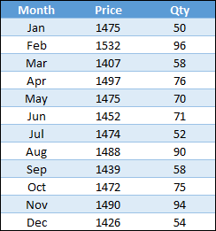
In the below example, we have 1658 as a normal average and 1445 as a weighted average. Let me clarify this difference by using two points.
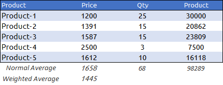
- First: If you multiply 1658 (average) by 68 (quantity) you will get 112742 which does not equal the total amount. But if you multiply 1445 (weighted average) by 68 (quantity) you will get 98289 which equals the total amount.
- Second: Product-1 has the lowest price and highest quantity whereas Product-4 has the highest price and lowest quantity.
While calculating the normal average you are not considering the quantity and if there is a change in quantity there will be no effect on the average price. And, in the weighted average, you can take quantity as a weight.
Step to Calculate Weighted Average in Excel
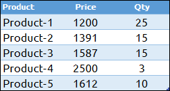
To calculate the weighted average, we are using the same data table that I have shown you in the above example.
Get the Excel File
Now, follow these two simple steps.
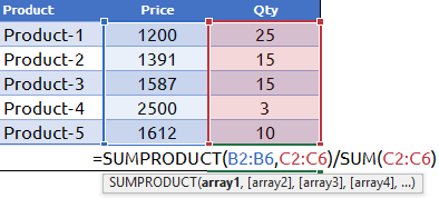
- In the C7 cell, enter following formula: =SUMPRODUCT(B2:B6,C2:C6)/SUM(B2:B6).
- Click OK.
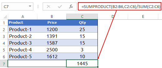
Now, you have 1445 as a weighted average of price and product. As I said, SUMPRODUCT is an effortless way to calculate the weighted average or mean in Excel. The best part about SUMPRODUCT is it can multiply and sum an array in a single cell.
How Does this Work
We need to break down this formula to understand it.
First, SUMPRODUCT will calculate the product of price and quantity for all the products and return the sum of all those. After that, some functions will give you the sum of the quantity. In the end, you will get the weighted average by dividing values from both functions.
Check this out: SUMPRODUCTIF
Calculate the Moving Weighted Average
Let’s go one step further. Let’s move to the data analysis part. Using the same formula, you can also calculate the weighted moving average.
Get the Excel File
Here are the steps:
- Enter the formula below in cell D4 and drag it to the end. =SUMPRODUCT(B2:B4,C2:C4)/SUM(C2:C4)
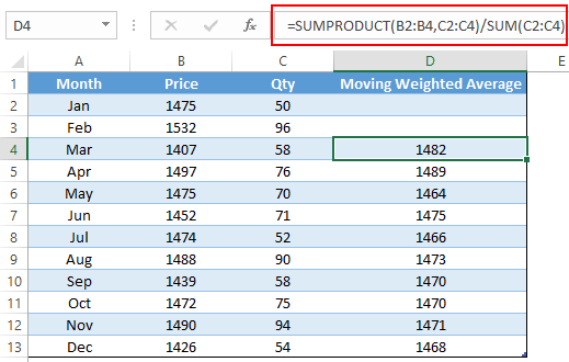
- Once you drag this formula, it will calculate the moving average on the basis of 3 months for each month.
How Does this Work
If you check the above snapshot, you will see that in cell D4, you have the moving average for January, February, and March, and in cell D5, you have the moving average for February, March, and April.
So, every time you move to a new month, you will get the moving average, including the current month and the last two months. When you drag down your formula, you just need to make your cell references relative.
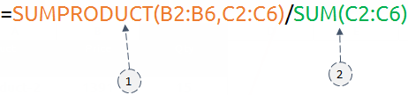
You’ve got conflicting formulas, the first step needs changing –
In the C7 cell, enter following formula.
=SUMPRODUCT(B2:B6,C2:C6)/SUM(B2:B6)
it should read
In the C7 cell, enter following formula.
=SUMPRODUCT(B2:B6,C2:C6)/SUM(C2:C6)
Nice to meet you, Puneet. Others have said it already, indeed a great post: short, clear but message comes across. Ordinary average is yuk, weighted average on the other hand… Something more useful. Versatile SUMPRODUCT to the rescue.
Yup
Great post ! Thank you!
Thanks for your words Kapil.
I have been looking for this technique for a long time! Thank you for explaining this.
Thanks for your words Lisa.
Hi, great post. Could you discuss using the sumproduct function for looking up 3 or 4 pieces of data and bringing back the sum of what matches these conditions. Thanks for your great work !
Hello Enna,
I hope this will help you.
https://excelchamps.com/excel-functions/