Have you ever selected a few cells in Excel and noticed that Excel instantly shows you the Sum, Average, and Count at the bottom?
That small area is called the Status Bar. And I must say, it is one of those Excel features that stays right in front of us, but most users do not use it fully.
In this tutorial, I’ll walk you through everything you can do with the Excel status bar — including worksheet views, zoom options, quick calculations, hidden customization options, and fixes for common problems like Sum not showing or the Status Bar missing.
Quick Answer: The Excel Status Bar is the thin bar at the bottom of the Excel window. It shows useful information such as Ready mode, quick calculations, worksheet view buttons, zoom controls, Caps Lock, Scroll Lock, and many other options that you can customize.
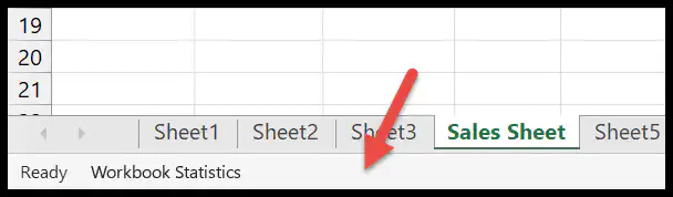
As you can see in the screenshot above, the status bar runs across the bottom of the Excel window. On the left side, it usually shows the current mode, such as Ready, Enter, or Edit. And on the right side, you usually see worksheet view buttons, zoom percentage, and the zoom slider.
Modes on Status Bar
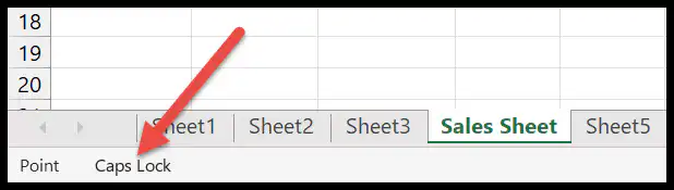
The left side of the status bar shows the current mode of Excel. These modes are small, but they tell you what Excel is doing at that moment.
Let me show you the four main modes you’ll commonly see there.
1. Ready
The Ready mode appears when Excel is waiting for your next action. This means you are not typing in a cell, editing a formula, or selecting a range for a formula.
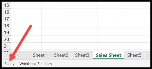
As you can see, Excel shows Ready at the bottom-left corner. Most of the time, this is the default mode you’ll see while working in a worksheet.
2. Enter
The Enter mode appears when you start typing a new value, text, or formula in a cell. At this point, Excel is waiting for you to finish entering the data.
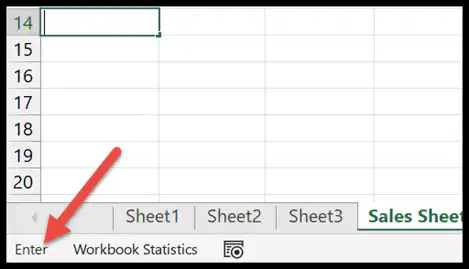
Once you press Enter, Excel confirms the entry and moves back to Ready mode.
3. Edit
The Edit mode appears when you are changing the content of an existing cell. You can enter this mode by double-clicking a cell or by pressing F2.
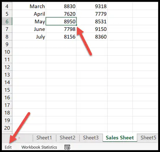
This is useful when you want to change only a small part of a formula or text without replacing the entire cell value.
If Excel is stuck in Edit mode and you want to cancel the change, press Esc. This takes you out of the cell without applying the edit.
4. Point
The Point mode appears when you are writing a formula and selecting cells or ranges to use inside that formula.
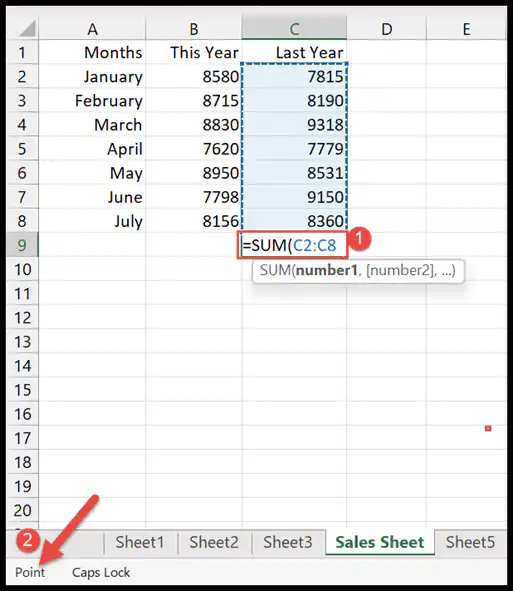
For example, when you type an equal sign and then select another cell, Excel changes to Point mode because you are pointing to a cell reference.

When teaching formulas, I always ask users to watch the status bar. If it says Point, Excel is waiting for you to select a cell or range for the formula.
Worksheet Views on the Status Bar
On the right side of the Excel status bar, you’ll find three worksheet view buttons. These buttons help you quickly change how your worksheet appears on the screen without going to the View Tab ➜ Workbook Views.
These three options are Normal View, Page Layout View, and Page Break Preview. Each one is useful in a different situation.
1. Normal View
The Normal View is the default worksheet view in Excel. It shows rows and columns in a simple grid so that you can enter and edit data easily.
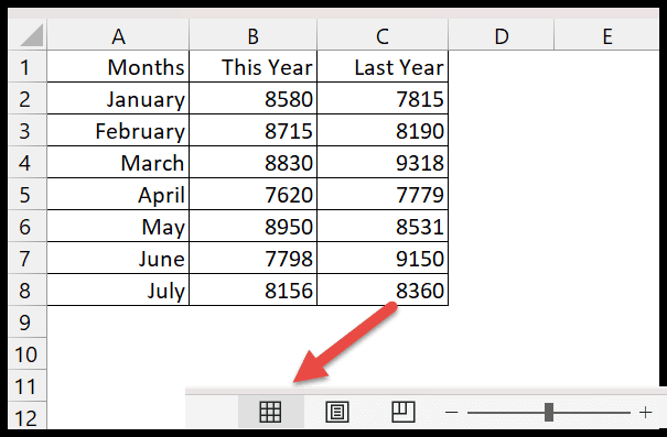
Most of the time, you’ll work in this view while creating datasets, writing formulas, or preparing dashboards.
2. Page Layout View
The Page Layout View helps you see how your worksheet will look when printed. It shows margins, headers, and footers directly on the screen.
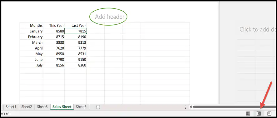
This view is extremely useful when you are preparing reports that you plan to print or share as PDFs.
You can also open this view from View Tab ➜ Page Layout if you prefer using the ribbon instead of the status bar.
3. Page Break Preview
The Page Break Preview shows where Excel will divide your worksheet into pages during printing. This makes it easier to adjust page breaks before printing the worksheet.
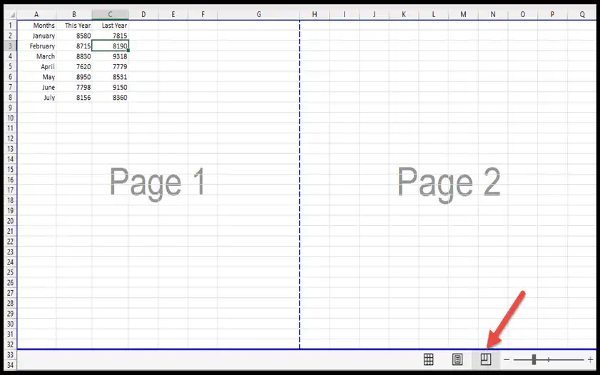
You can also drag the blue lines in this view to adjust the page breaks manually.
Whenever I prepare printable reports, I switch to Page Break Preview first. It saves time because I can control exactly how many pages the worksheet will use before printing.
Zoom Slider on the Status Bar
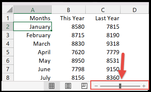
The Zoom Slider is one of the most frequently used options on the Excel status bar. It appears at the bottom-right corner of the Excel window and allows you to quickly adjust the worksheet view size.
You can use the minus (-) and plus (+) buttons to zoom out or zoom in. And you can also drag the slider left or right to adjust the zoom level smoothly.
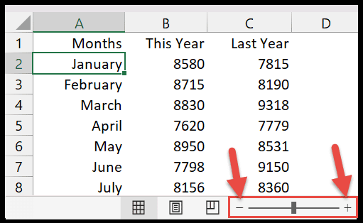
When you move the slider toward the plus sign, Excel increases the zoom level so you can look at data more closely. And when you move it toward the minus sign, Excel reduces the zoom level so that you can see more data on the screen.
This adjustment only changes how the worksheet appears on your screen. It does not change the actual size of the data or affect printing.
You can also zoom in and out quickly by holding Ctrl and scrolling your mouse wheel.
When I review large datasets, I zoom out first to see the overall structure and then zoom in on specific columns. It helps me understand the layout faster before starting analysis.
Quick Calculations Using the Status Bar (Without Writing Formulas)
One of the most powerful uses of the Excel status bar is that it can instantly calculate results for selected cells — without writing any formula.
When you select a range that contains numbers, Excel automatically shows calculations like Sum, Average, and Count at the bottom-right side of the status bar.
This helps you quickly verify totals and statistics without inserting formulas into your worksheet.
Steps to see quick calculations from the status bar:
- Select the cells that contain numeric values.
- Look at the bottom-right corner of the Excel window.
- You’ll immediately see results like Sum, Average, and Count.
Available Quick Calculation Options
You can enable multiple calculation options from the status bar depending on what type of summary you want to see.
Option |
What It Shows |
When to Use |
|---|---|---|
Average |
The average of selected numeric cells |
Quickly check the mean value of sales, marks, or measurements |
Count |
Total non-empty selected cells |
Check how many cells contain any value |
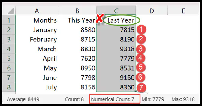
Numerical Count |
Only counts numeric cells |
Useful when your data contains both text and numbers |
Sum |
Total of selected numeric values |
Quickly verify totals without formulas |
Minimum |
Lowest value from selected cells |
Identify smallest number instantly |
Maximum |
Highest value from selected cells |
Identify largest number instantly |
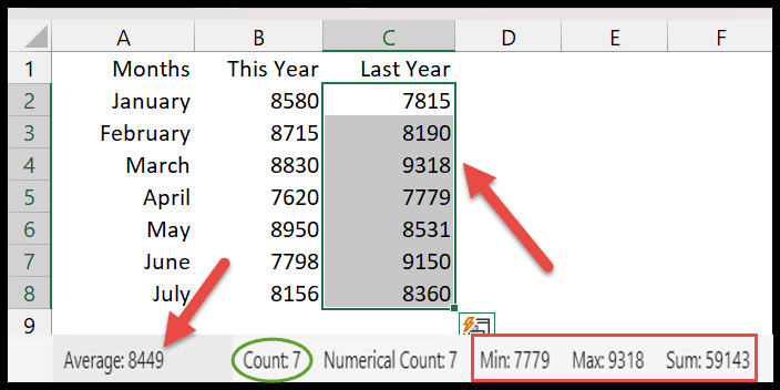
If you cannot see Sum, Average, or Count on the status bar, right-click the status bar and enable these options from the list.
Before writing any SUM formula, I always select the range and check the status bar first. Many times, this quick check saves me from inserting unnecessary formulas.
Customize the Status Bar in Excel
The Excel status bar is not fixed. You can customize it based on the type of information you want to see while working in a worksheet.
By default, Excel shows some options automatically. But there are many more options available that you can enable anytime.
Steps to customize the status bar:
- Right-click anywhere on the status bar.
- A customization menu will open.
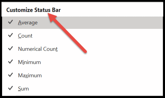
- Select the options you want to display.
- The moment you select an option, Excel shows it on the status bar.
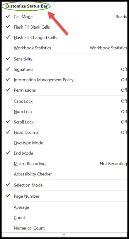
As you can see in the screenshot above, Excel provides multiple options that you can enable or disable depending on your requirement.
Commonly Used Status Bar Options
Below is a list of some useful options that you can activate from the customization menu.
Option |
What It Does |
When It Helps |
|---|---|---|
Average |
Shows average of selected cells |
Quickly analyze numeric datasets |
Count |
Counts non-empty cells |
Check filled entries instantly |
Numerical Count |
Counts numeric-only cells |
Useful for mixed datasets |
Minimum |
Shows lowest value |
Find smallest number quickly |
Maximum |
Shows highest value |
Find largest number quickly |
Sum |
Shows total of selected cells |
Verify totals instantly |
Workbook Statistics |
Displays workbook details |
Audit workbook structure quickly |
Caps Lock |
Shows Caps Lock status |
Avoid typing mistakes |
Num Lock |
Shows Num Lock status |
Prevent number-entry issues |
Scroll Lock |
Shows Scroll Lock status |
Fix arrow key movement problems |
Selection Mode |
Shows selection extension mode |
Track extended selections |
Macro Recording |
Indicates macro recording status |
Avoid recording mistakes |
View Shortcuts |
Shows worksheet view buttons |
Switch views quickly |
Zoom Slider |
Shows zoom adjustment slider |
Adjust worksheet visibility easily |
You only need to enable an option once. After that, Excel remembers your choice and keeps it active for future workbooks.
I always enable Numerical Count along with Sum. When checking datasets received from clients, this quickly tells me whether the column contains unexpected text values.
Fix: Excel Status Bar Sum Not Showing
Sometimes when you select cells in Excel, the Sum, Average, or Count does not appear on the status bar. This is one of the most common issues users face while working with quick calculations.
The good news is that this problem usually happens because the calculation options are not enabled on the status bar.
Steps to fix the Sum not showing in the status bar:
- Select any range of numeric cells.
- Right-click on the status bar.
- From the menu, enable Sum, Average, or Count.
- Now look again at the bottom-right corner of the Excel window.
The moment you enable an option from the list, Excel immediately starts showing that calculation on the status bar.
If Sum Still Does Not Appear
If enabling the option does not solve the problem, then the selected cells may contain values stored as text instead of numbers.
Check if numbers are stored as text:
- Select the cells.
- Look for a small green triangle in the corner of the cells.
- If visible, click the warning icon.
- Select Convert to Number.
Once the values are converted to numbers, Excel starts showing the correct Sum and other calculations on the status bar.
If your selection contains only text values, Excel will not display Sum because Sum works only with numeric data.
If the status bar shows Count but not Sum, that usually means the numbers are stored as text. I always check this first before troubleshooting anything else.
Workbook Statistics from the Status Bar
Workbook Statistics is one of the most useful options you can add to the status bar. It gives you a quick summary of the active sheet and the entire workbook.
To enable it, right-click the status bar and select Workbook Statistics from the list.
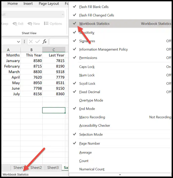
Once it appears on the status bar, click Workbook Statistics, and Excel opens a dialog box with details about your worksheet and workbook.
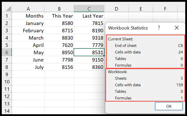
This dialog box can show details like the number of sheets, cells with data, tables, formulas, charts, and other workbook-level information.
Use Workbook Statistics when you receive a file from someone else and want to quickly understand how large or complex the workbook is.

Before cleaning or auditing a workbook, I open Workbook Statistics once. It gives me a quick idea of how many formulas, tables, and used cells I’m dealing with.
Caps Lock, Num Lock, and Scroll Lock on the Status Bar
The Excel status bar can also show whether Caps Lock, Num Lock, or Scroll Lock is turned on. These small indicators are useful because they explain why Excel is behaving differently while you type or move around the worksheet.
To show these indicators, right-click the status bar and make sure Caps Lock, Num Lock, and Scroll Lock are enabled in the customization menu.
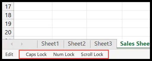
As you can see in the screenshot above, Excel displays the lock indicators on the left side of the status bar when these keys are active.
Why Scroll Lock Matters in Excel
Scroll Lock is the most confusing one for many users. When Scroll Lock is on, the arrow keys may move the worksheet view instead of moving from one cell to another.
Steps to turn off Scroll Lock:
- Check the status bar to confirm if Scroll Lock is active.
- Press the Scroll Lock key on your keyboard.
- If your keyboard does not have this key, open the Windows On-Screen Keyboard.
- Click ScrLk to turn it off.
If your arrow keys are not moving between cells, check the status bar first. In many cases, Scroll Lock is the reason.
Whenever someone tells me their arrow keys are not working in Excel, I first ask them to look at the status bar. If Scroll Lock is visible there, the fix is usually just one key press.
Selection Mode on the Status Bar
The Selection Mode indicator on the Excel status bar shows how Excel is currently selecting cells when you move using the keyboard. This is especially helpful when working with large datasets where extended selection is required.
Excel has three main selection modes that can appear on the status bar: Ready, Extend Selection, and Add to Selection.
Different Selection Modes Explained
Mode |
What It Means |
How It Helps |
|---|---|---|
Ready |
Normal selection behavior |
Default working mode in Excel |
Extend Selection |
Expands selection using arrow keys |
Select large ranges quickly |
Add to Selection |
Adds multiple ranges to selection |
Select non-adjacent ranges easily |
You can activate these selection modes directly using keyboard shortcuts while working in Excel.
Keyboard shortcuts for selection modes:
- Press F8 to enable Extend Selection mode.
- Press Shift + F8 to enable Add to Selection mode.
- Press Esc to return to Ready mode.
Extend Selection mode helps you select large datasets faster without holding the Shift key continuously.
I often use F8 (Extend Selection) when reviewing large tables. It makes selecting long ranges much smoother compared to dragging with the mouse.
Macro Recording Indicator on the Status Bar
The Excel status bar can also show whether Macro Recording is currently active. This is very helpful when you are working with VBA macros and want to make sure Excel is recording your actions correctly.
To display this indicator, right-click the status bar and enable the Macro Recording option from the customization menu.
Once enabled, Excel shows a small recording indicator on the status bar whenever macro recording starts. This confirms that Excel is capturing each step you perform.
Why This Indicator is Useful
When recording macros, it’s easy to forget whether recording is currently active or not. The status bar indicator helps you avoid missing important steps or accidentally recording unnecessary actions.
Typical workflow when recording a macro:
- Go to the Developer Tab.
- Click Record Macro.
- Check the status bar to confirm recording is active.
- Perform the required steps.
- Click Stop Recording when finished.
If you forget to stop recording, Excel continues capturing every action, which may create unnecessary steps inside your macro.
Worksheet View Shortcuts on the Status Bar
The Excel status bar also includes Worksheet View Shortcuts that allow you to quickly switch between different worksheet layouts. These shortcuts are located near the bottom-right corner of the Excel window.
Instead of going to the View Tab on the ribbon, you can change the worksheet view instantly using these buttons.

Available Worksheet View Options
View Mode |
What It Does |
Best Use Case |
|---|---|---|
Normal View |
Standard worksheet editing layout |
Daily data entry and analysis |
Page Layout View |
Shows how the sheet appears when printed |
Adjust margins, headers, and footers |
Page Break Preview |
Displays page break boundaries |
Control print area across multiple pages |
These shortcuts help you switch views instantly without interrupting your workflow. This is especially useful when preparing worksheets for printing or reviewing page layouts.
Use Page Break Preview when printing large reports. It helps you adjust page boundaries visually before printing.
In the End
The Excel Status Bar is one of those small features that many users ignore, but once you start using it properly, it can save a lot of time during everyday work. It helps you quickly check calculations, switch worksheet views, monitor typing modes, and adjust zoom without opening extra menus.
You can also customize the status bar to show only the information you actually need. Whether you are reviewing datasets, building dashboards, or checking totals quickly, the status bar works like a smart assistant at the bottom of your screen.
If you frequently work with large datasets, enable Sum, Average, Minimum, Maximum, and Numerical Count together on the status bar. This turns it into a quick analysis panel without writing a single formula.
When reviewing client files, I always select entire columns once to quickly check Sum and Numerical Count on the status bar. It helps me instantly detect missing numbers or unexpected text values before starting deeper analysis.
Frequently Asked Questions About the Excel Status Bar
What is the Status Bar in Excel?
The Status Bar is the horizontal strip at the bottom of the Excel window that shows useful information like Sum, Average, Count, Zoom level, worksheet view shortcuts, and typing modes such as Caps Lock or Num Lock.
Can I customize the Excel Status Bar?
Yes. You can customize the Status Bar by right-clicking anywhere on it and selecting the options you want to display, such as Sum, Numerical Count, Minimum, Maximum, or Workbook Statistics.
Why is Sum not showing on the Status Bar?
If Sum is not showing, either the option is disabled or the selected values are stored as text instead of numbers. Right-click the Status Bar and enable Sum, then check whether the selected cells contain numeric values.
How do I restore the Status Bar if it disappears?
Go to File ➜ Options ➜ Advanced, scroll to the Display section, and enable Show Status Bar. This restores the Status Bar at the bottom of the Excel window.
Does the Status Bar work in Excel Online?
Yes, but with limited functionality. Excel Online shows basic calculations like Sum and Average, but some advanced Status Bar customization options are available only in the desktop version of Excel.

Last updated: