How to Apply Accounting Number Format in Excel

Microsoft Excel is widely used for business and accounting purposes and when users use Excel for accounting purposes, their data sets usually have a set of numbers.

And they might want to convert the numbers from standard number format to accounting number format to make the data set clearer and more suitable for accounting.

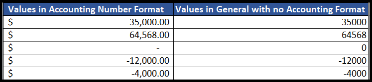
The accounting number format converts the general number format by adding the currency symbol at the extreme left side of the cell, thousand number separators, and two decimal places (0.00) at the end of each number.

The accounting number format also displays the zero (0) value as a dash “- “.

We have some quick and easy steps below for you to apply the accounting number format in Excel.

Apply Accounting Number Format using Accounting Number Format Button

1. First, select the cells or range with the numbers which you want to format.
2. After that, go to the “Home” tab and then click on the “Accounting Number Format” button.
3. Now click on the accounting format with the currency symbol from the drop-down list you want to add.
   
4. At this point, your selected cells or range has changed to “Accounting Number Format” by adding currency symbol, thousand numbers separators, and two decimal places to the number values.
   
5. To increase or decrease the decimal values to the numbers, you can do using the decimals increase and decrease icons under the “Number” group on the ribbon.
   

Apply Accounting Number Format Using the Drop-Down in the Number Group

1. First, select the cells or range with the numbers which you want to format.
2. After that, go to the “Home” tab and then click on the drop-down arrow under the “Number” group on the ribbon.
   
3. Now, click on the “Accounting” option from the drop-down list.
   
4. At this point, your selected cells or range has changed to “Accounting Number Format” by adding currency symbol, thousand numbers separators, and two decimal places to the number values.
   

As you saw in this method, we don’t have an option to select the accounting format with the choice of currency symbols.

So there might be a possibility that the accounting number format using this drop-down option will display the currency symbol of your country’s currency which could be the default set currency of your system.

Apply Accounting Number Format Using the Format Cells Option

With this method of accounting number format, users can change the set default currency symbol of your system and can select the currency symbol from multiple currency symbols based on different countries currencies.

1. First, select the cells or range with the numbers which you want to format, and then right click on your selection.
2. After that, select the “Format Cells” option from the drop-down menu and you will get the “Format Cells” dialog box opened.
   
3. Now, select the “Number” tab and under the “Category” select the “Accounting” option.
4. Now, click on the “Symbol” drop-down arrow and scroll the currency options downwards and select the one which you want.
5. In case, you want to increase or decrease the decimal values to the numbers, you can do the same using the “Decimal Places” up and down arrow.
6. Once done, click OK.
   
7. At this point, your selected cells or range has changed to “Accounting Number Format” by adding the currency symbol you just selected with the thousand numbers separators and two decimal places to the number values.