And you will be amazed that I have got seven different ways you can use to deal with negative numbers. Last week, I got an email from one of my subscribers with a question.
Hey Puneet, how many methods do we have to convert a negative number into a positive one?
You know, the thing for which he asked is a common kind of task. I am sure, this often happens to you, when you get some negative numeric values, and after that, you convert them into positive ones.
There is no #rocketscience in this. But have you ever checked how my different methods you have to do this? Well, I am always curious to know about different methods to do a task in Excel.
So this time I grabbed a paper and listed all the methods which I can use to convert a negative number into a positive. So today in this post, I’d like to share all those methods with you.
Let’s get started.
1. Multiply with Minus One to Convert a Positive Number
Unlike me, if you are good at maths, I am sure you know that when you multiply two minus signs with each other, the result is always positive. So you can use the same method in excel to convert a negative number into a positive.
All you have to do is just multiply a negative value with -1 and it will return the positive number instead of the negative.
=negative_value*-1Below you have a range of cells with negative numbers. So to convert them into positive you just need to enter the formula in cell B2 and drag it up to the last cell.

If you have mixed numbers (both positive and negative) then you can use the below method instead.
=IF(A1<0,A1*-1,A1)2. Convert to an Absolute Number with ABS Function
Turning a negative number into a positive is quite easy with ABS. This function is specifically for this task.
Quick Intro: It can convert any number into an absolute number. In simple words, it will return a number after removing its sign.
=ABS(number)You just have to refer a negative number into the function and it will turn it into a positive value.
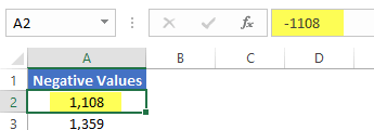
- In the below example, you have negative values from range A2:A11.
- Enter
=ABS(A2)into B2 and drag it up to the last cell.

This function works even when you have mixed numbers (both positive and negative).
3. Multiple Using Paste Special
Let’s think about a different situation where instead of getting positive numbers in a different column you need them in the same column.
And for this, you can use the paste special option. Wondering how? Let me tell you. In the paste special option, there are “operation” options that you can use to perform some simple calculations. You can use these same options to make negative numbers positive without using any formula or adding any extra column. Just follow these steps.

- First of all, in any cell in your worksheet, enter -1.
- After that, copy it.
- Now, select the range of cells in which you have negative numbers.
- Right-Click ⇢ Paste Special ⇢ Operations ⇢ Multiply.
- In the end, click OK.
All the negative numbers are converted into positive ones.
The only thing you need to take care of is that this is not a dynamic method. So, you need to do it again and again if you frequently update your data. But this method is quick and easy to use, and you don’t need any formula.
4. Remove the Negative Sign with Flash Fill
I am sure you have used flash fill once in your lifetime and if not, you must use it, it’s a game-changer. This is an insane method to turn negative numbers into positive ones, here are the steps.

- First of all, in cell B2, enter the positive number for the negative number you have in cell A2.
- After that, come to cell B3 and press the shortcut key Ctrl + E.
- At this point, in the B column, you have all the numbers in positive form.
- Now, click on the small icon you have on the right side of column B and select “Accept Suggestions”.
Congratulations, you have converted all the negative numbers into positive ones with flash fill.
This method is also not a dynamic one, but quick and easy to use.
5. Apply Custom Formatting to Show as Positive Numbers
This is also a possibility that instead of converting a negative number you just want to show it as a positive number. And in this situation, you can use custom formatting. Here are the steps to this.
- First of all, select the range of the cells you need to convert into positive numbers.
- After that, press the shortcut key Ctrl + 1. It will open the custom formatting options.
- Now, go to “Custom” and in the type input bar, enter “#,###;#,###”.
- In the end, click OK.

This will show all the negative numbers as positive. But, in actuality, these all are still negative numbers, just formatting is changed.
If you select a cell and look at the formula bar, you can check, that it’s still a negative number. So, when you use it in further calculation it will act as a negative number.
6. Run a VBA Code to Convert to Positive Numbers
If you are a VBA lover then you can use a simple code to reverse the sign of negative numbers instantly.
Sub numberP2N()

Dim myCell As Range

For Each myCell In Selection

    If myCell.Value <> "" Then

        If IsNumeric(myCell.Value) Then

            myCell.Value = Abs(myCell.Value)

        End If

    End If

Next myCell

End Sub
To use this code, you just need to select the range of negative numbers and run this macro.
First, it will check each cell of selection if there is a numeric value in it or not and then convert it to a positive value.
Once you run this code, you can’t undo your action.
Related: VBA Tutorial
7. Use Power Query to Convert Get Positive Numbers
Yes, you can use a power query to convert a negative number into a positive number and the best part is it’s a one-time setup. Just follow these simple steps.
- First of all, select any of the cells from the data range where you have negative numbers.

- After that, go to the Data tab ➜ From Table.

- It will convert the range into a table and load it in the power query editor.

- Now, right-click on the column, and go to Transform ➜ Absolute Value.

- In the end, in the power query editor, go to Home Tab ➜ Close ➜ Close and load.

Related: Power Query Tutorial
Conclusion
As I said, to turn a negative number into a positive number you don’t need to use rocket science. Even one method can be sufficient, but I have listed all these methods to help you to handle different situations.
I am sure you found all these methods helpful, but now, you have to tell me one thing.
Do you know any other method for this? Please share your views with me in the comment section. I’d love to hear from you and please don’t forget to share it with your friends, I am sure they will appreciate it.
Great tutorial! I never realized how simple it could be to convert negative numbers into positives in Excel. Your step-by-step instructions were really helpful. Thanks for sharing!
Thanks for help me
Your macro can be simplified to a non-looping one-liner…
Sub MakeNegPos()
Selection.Replace “-“, “”, xlPart
End Sub
Note: The selection does not have to be contiguous.
A simple “Desi Upchaar” is here,
Go to Find and Replace and type “-” in find,
then replace with none. Now, “-” sign is
removed from negative numbers.
This is a static method, not dynamic.
Nitin Shukla.
This was a great suggestion thanks!
This is very useful and thank you
Thanks Puneet,
Informative
using power query to get positive numbers is a very good option when you need absolute values for analysis. Thanks for the help
Congratulations and thanks.
There is an 8th method with Paste Special
A very simple method that I used often, hope you like it ,
you can use “find & replace” option . you can find “-” & replace it with a blank ( like ” ” )
That’s so nice of you. Thank you so much. 🙂
Thanks Puneet.
How i can convert the only negative numbers. And posative must be zero Like this example.
A. B.
-2. 2
33. 0
Use VBA or an conditional formula.
if(A1>0, “0”, Abs(A1)
Where A1 is the cell containing Question Value
Thank you, Puneet.
Great methods.
However, some of the techniques might not work as expected when you have mixed negative and positive numbers.
Yes, #1 and #3 will not work.
Thanks Puneet !!
I’m so glad you found it useful.