

COUNTIFS applies AND logic across its conditions, so it can’t count “Facebook or Twitter” from one column on its own. The fix is to pass both values as an array constant and wrap the whole thing in SUM: =SUM(COUNTIF(B2:B51,{"Facebook","Twitter"})). COUNTIF runs once for each value in the curly brackets, returns a count for each, and SUM adds them together.
To pull the criteria from cells instead of typing them, point at the range and enter it with Ctrl+Shift+Enter in Excel 2019 or earlier: =SUM(COUNTIF(B2:B51,E1:E3)) — in Excel 365 a plain Enter works. There’s also a non-array route: =SUMPRODUCT((B2:B51="Facebook")+(B2:B51="Twitter")), where the plus sign is the OR.
One thing to watch: with overlapping conditions this double-counts, so if a row could match both criteria, use SUMPRODUCT with –((B2:B51=”A”)+(B2:B51=”B”)>0) instead.
How to Use COUNTIF/COUNTIFS OR
The data below lists 50 people and the social platform each one uses. Names are in column A, platforms in column B.

To count how many people chose Facebook or Twitter — either one counts — enter this in a cell and press Enter.
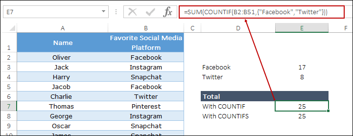
You get 25 — 17 people on Facebook and 8 on Twitter. COUNTIFS returns the same number, and the order of the values inside the brackets makes no difference.
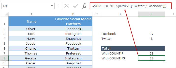
Curly brackets you type yourself are an array constant, and this formula takes a plain Enter in every version of Excel, right back to 2010. Curly brackets Excel adds for you mean something different — that comes up in the next method.
How It Works
SUM is doing the OR part, not COUNTIF. Split the formula into three pieces, and it’s obvious.
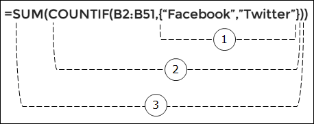
- The array constant {“Facebook”,”Twitter”} holds both criteria in one argument.
- COUNTIF runs once for each value in that constant and returns two numbers instead of one — {17,8}.
- SUM adds those two numbers into a single result, 25.
That’s why the same structure works with COUNTIFS. You’re not asking either function to handle OR — you’re running it twice and adding the answers.
Select just the COUNTIF(B2:B51,{“Facebook”,”Twitter”}) part inside the formula bar and press F9. Excel shows you the two counts before SUM collapses them. It’s the fastest way to check which criteria value is returning zero.
Use a Range of Cells for the Criteria
Typing the values inside the formula is fine for two or three fixed values. But if you want to change the criteria without editing the formula, type them in cells, say E1:E3, and refer to that range instead of the array constant:
=SUM(COUNTIF(B2:B51,E1:E3))
In Microsoft 365 and Excel 2021, a plain Enter works. In Excel 2019 and earlier, you need to enter it with Ctrl + Shift + Enter, and Excel adds the curly brackets around the formula for you. These are the brackets the note above talks about: they show that the formula was entered as an array formula. If you press only Enter in an older version, the formula can return the #VALUE! error or count only one of the values.
If you don’t want to remember that, use SUMPRODUCT in place of SUM. It takes a plain Enter in every version:
=SUMPRODUCT(COUNTIF(B2:B51,E1:E3))
Keep the criteria list free of blank cells. Microsoft notes that COUNTIFS treats an empty criteria cell as 0, so a blank in E1:E3 counts cells that hold 0, not empty cells.
And if you want to count each row only once, even when your list has overlapping values, use MATCH. It checks every cell in B2:B51 against the list, and ISNUMBER returns TRUE when the cell is found:
=SUMPRODUCT(--ISNUMBER(MATCH(B2:B51,E1:E3,0)))
The SUMPRODUCT Alternative
SUMPRODUCT gets you the same 25 without SUM, without an array constant, and without Ctrl + Shift + Enter in any version.
Each comparison tests all 50 rows and returns TRUE or FALSE for every one. The plus sign adds the two result sets row by row, which converts the TRUEs to 1s along the way, and SUMPRODUCT totals them.
I reach for this one when the criteria have to be built inside the formula — a comparison, a date test, a wildcard match with SEARCH — because COUNTIF’s criteria argument gets awkward fast once you go past plain text.
When Your Criteria Overlap (Avoid Double Counting)
Every formula above counts each criterion separately and then adds the results. That’s correct as long as a row can match only one of your values. The moment a row can match both, it gets counted twice.
In the sample data, each person lists a single platform, so 25 is right. But if column B held more than one platform per person, or you were testing two conditions that can both be true, you’d need to test the combined result against zero.
Adding the two comparisons gives 0, 1, or 2 for each row. The >0 test flattens anything above zero back to a single TRUE, so a row that matches both still counts once. The double minus converts those TRUEs to 1s so SUMPRODUCT can add them.
Leave out the >0 and the formula still returns a number — just a wrong one. There’s no error to catch it. I shipped that mistake in a client report once and only found it because the total came out higher than the row count.
OR Logic Across Two Different Columns
Everything so far tested one column. When your two conditions sit in different columns, COUNTIFS on its own can’t do it — it will only give you the AND version — so use SUMPRODUCT.
Say column B holds the main platform and column C holds a second choice. To count the people who picked Facebook in either column:
The >0 matters more here than anywhere else on this page, because someone can easily have Facebook in both columns and you only want to count that person once.
For the opposite job — both conditions must be true — COUNTIFS is the right tool, and this is exactly what its AND logic is for:
If you’d rather stay with COUNTIF, you can count each column separately and then take away the rows that match in both, so nobody is counted twice:
=COUNTIF(B2:B51,"Facebook")+COUNTIF(C2:C51,"Facebook")-COUNTIFS(B2:B51,"Facebook",C2:C51,"Facebook")
It gives the same result as the SUMPRODUCT formula with the >0 test, but it gets long quickly when you add more values.
OR and AND in the Same Formula
You can also mix both kinds of logic. Let’s say you want to count the people whose main platform is Facebook or Twitter and whose second choice is Instagram. Use the array constant for the OR part and a normal criteria pair for the AND part:
=SUM(COUNTIFS(B2:B51,{"Facebook","Twitter"},C2:C51,"Instagram"))
COUNTIFS runs once for each value in the array constant, each time with the Instagram condition, and SUM adds the two counts. The SUMPRODUCT version of the same count is below:
=SUMPRODUCT(((B2:B51="Facebook")+(B2:B51="Twitter"))*(C2:C51="Instagram"))
Here, the plus sign works as OR and the multiplication works as AND.
OR Logic with Wildcards and Numbers
The values in the array constant are normal COUNTIF criteria, so you can use wildcards in them. The formula below counts every cell that starts with Face or Twit, which also catches a value like “Facebook ” with a trailing space:
=SUM(COUNTIF(B2:B51,{"Face*","Twit*"}))
And you can use comparison operators the same way. For numbers in D2:D51, this formula counts the values below 100 or above 500:
=SUM(COUNTIF(D2:D51,{"<100",">500"}))
Just make sure the conditions can’t overlap (like “>100” and “>500”), or a value that matches both gets counted twice.
Which Method Should You Use?
Method | Formula | How to enter | When to use |
|---|---|---|---|
Array constant |
=SUM(COUNTIF(B2:B51,{"Facebook","Twitter"})) |
Enter, all versions |
Two or three fixed values you won’t change |
Criteria from cells |
=SUM(COUNTIF(B2:B51,E1:E3)) |
Enter in 365 and 2021; Ctrl + Shift + Enter in 2019 and earlier |
Criteria you want to change without editing the formula |
SUMPRODUCT |
=SUMPRODUCT((B2:B51="Facebook")+(B2:B51="Twitter")) |
Enter, all versions |
Conditions built inside the formula, or two different columns |
SUMPRODUCT with >0 |
=SUMPRODUCT(--((B2:B51="Facebook")+(B2:B51="Twitter")>0)) |
Enter, all versions |
Any time a row could match both conditions |
Frequently Asked Questions
Why does my array formula return zero?
It’s almost always a spelling or spacing mismatch between your criteria and the cell values — COUNTIF matches the whole cell, so a trailing space in column B means no match. Test one value on its own with =COUNTIF(B2:B51,”Facebook”) first. If that returns zero too, run =TRIM() over your data. If it returns a number but the combined formula doesn’t, the problem is how the formula was entered, not the data.
Do I need Ctrl + Shift + Enter in Microsoft 365?
No. Dynamic arrays handle it, so a plain Enter works for every formula on this page. In Excel 2019 and earlier, you still need Ctrl + Shift + Enter for the version that pulls criteria from a range of cells. The array constant version and both SUMPRODUCT versions take a plain Enter in every version.
Why does Excel print my formula as text with the curly brackets?
Because you typed the outer curly brackets yourself. Those are Excel’s way of showing you a formula that was entered as an array — they’re display, not input. Retype the formula without them and press Ctrl + Shift + Enter, and Excel puts them back on its own.
How do I avoid double counting?
Wrap the added comparisons in a >0 test inside SUMPRODUCT. Adding two conditions gives a row that matches both a value of 2; the >0 test turns that back into a single TRUE, so the row counts once.
How Do I Count Cells That Are Not Facebook or Twitter?
Use COUNTIFS with a “not equal to” condition for each value. Here, both conditions must be true, so a row is counted only when it’s neither Facebook nor Twitter:
=COUNTIFS(B2:B51,"<>Facebook",B2:B51,"<>Twitter")
Keep in mind that this also counts blank cells in the range.
How Many Values Can I Put in the Array Constant?
There’s no small limit, but the formula gets hard to read after four or five values. For a longer list, put the values in cells and use SUMPRODUCT(COUNTIF(B2:B51,E1:E10)), so you can change the list without touching the formula.
Conclusion
OR logic in COUNTIF and COUNTIFS comes down to one idea: count each value separately, then add the counts. SUM around COUNTIF does that with fixed values, a criteria range does it with values you can change, and SUMPRODUCT does it when the conditions are more than plain text or sit in different columns.
The only trap is overlap. If a row can satisfy two of your conditions, add the >0 test before you trust the number. That’s all.
Read next: OR Logic in SUMIF and SUMIFS and COUNTIF Between Two Numbers.
Updated

Great post! The examples you provided on using OR logic in COUNTIFS really clarified how to count multiple values effectively. I appreciate the step-by-step approach—it makes it so much easier to apply in my own spreadsheets. Thank you for sharing!
Great job breaking down the use of OR Logic in COUNTIFS and COUNTIF formulas! I’ve been struggling to use these functions effectively, but your post has really helped clarify things for me.
Hi Puneet, Dynamic count doesn’t work for me. I am using office 365. Believe we need curly brackets at the front and at the end? It just print {=SUM(COUNTIFS(B2:B51,Named_Range))} as it is. Without curly brackets it just give zero.
Hi
I had the same issue initially but what you have to do is type the formula =SUM(COUNTIFS(B2:B51,Named_Range)) then instead of just hitting enter at the end rather hit ctrl + shift +enter … this will populate your cell with the answer and auto enclose your formula with {}
I’m confused…is the formula COUNTIF or COUNIF? My version of Excel (Excel 2016) does not recognize COUNIF.
=SUMPRODUCT(–(B:B=”Facebook “) +(B:B=”Twitter ” ))
This above formula can be used for above questions..
No words to says to be frank I don’t even know we can use countif with sum formula. Amazing Puneet. I hope you will grab more like these amazing feature into our purse
How would you do this inVBA?
I don’t know how but you do guess what we have in mind to look for the solutions which we require most. Plus your tips guides me to explore new avenues regarding Excel problem solving methods. Please do keep up with the good work.
I am enjoying weekends by applying your excel tips which I received by email, it’s very useful and apply it in my daily at work and remind functions of excel. I appreciate your work, God bless you always.
Thanks, Najib. Your words are blessings.
Good post! But the article’s title and conclusion, as well as a lot of verbiage in between, are about COUNTIF/COUNTIFS “OR”. I can’t find “OR” in any of the example formulas. Am I missing something?
ha ha ha You gave me a laugh.
I think I missed something while explaining, I’ll try to improve. But the thing is it’s not about combing COUNTIF with OR but adding a OR effect in it.
Thanks for the reply. I’m looking forward to learning more about COUNTIF…OR. Also, thanks for the many email newsletters that I’ve found extremely useful. I’ve been an Excel developer for 19-plus years and I continue to be amazed by the things you do with formulas. Keep ’em coming!
You’re Welcome.
Thank you for the sample that you have noticed.
You’re Welcome
Hello Ponit Sir, the way you explain Excel, it is a very good way. This makes us understand easily. I am very grateful to you that you know the excellence of Excel in such a nice and easy way.
Thank you for these kind words
punnet sir,
pls try to post offset function of excel.
Sure.