

Select the range, go to Home → Conditional Formatting → New Rule → Format only cells that contain, choose Blanks in the first box, set a fill under Format and click OK. The colour disappears as soon as a value goes in.
To colour the whole row when a key column is empty, use Use a formula to determine which cells to format with =$C2="", applied to the full data range starting in row 2. To count the gaps, use =COUNTBLANK(A2:F100).
For a one-off fill, select the range, press F5, click Special, choose Blanks and apply a fill colour. This colour stays after the cells are filled in.
The methods don’t agree on what counts as blank. The Blanks rule and =A2="" also catch formulas that return "", but Go To Special → Blanks and ISBLANK() find only truly empty cells. Cells holding a space look empty but aren’t; the Blanks rule catches them, while =A2="" doesn’t.
It’s hard to recognize blank cells in large data because a blank cell is just a white cell without any value. In most cases, blank cells represent some sort of gap or missing data, or a formula returns an empty string, resulting in a blank-looking cell.
And that’s why it’s recommended to highlight these cells with a color so that we can recognize them.
You might be wondering: Which is the best method to find and highlight cells that are blank? But here’s the kicker: It depends on you, as there is more than one way to do this, and you can use any of these ways to get your work done. All of these methods are unique.
So today, in this post, I’d like to share with you 3 different methods which you can use to highlight the blank cells in Excel. So let’s get started.
Here we have the below table, where we have some empty cells. You can download it from here to follow along.
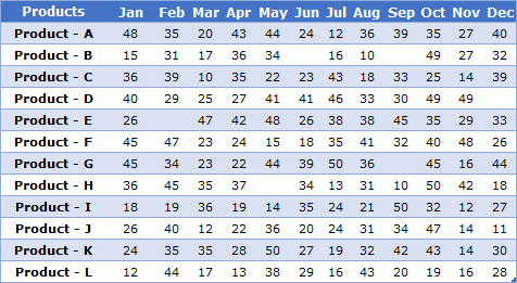
Highlight Blank Cells with GoTo Special
If you want to apply color to all the blank cells in a range, the Go To Special option can be an easy-to-use way. This method is simple: Select all the blank cells and apply cell color. Yes, that’s it. Below are the steps you need to follow to highlight all the blank cells.
- First of all, select your entire data.

- Go to Home Tab ➤ Find & Select ➤ Click on “Go To Special”.

- From the Go To Special window, select “Blanks” and click OK. (It will select all the blank cells in the table.)
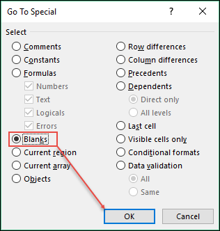
- After that, go to the Home tab and apply the fill color to highlight the cells.

If you want to use a dynamic method, use conditional formatting, which is the next method.
You can also open Go To Special with the keyboard: press F5 (or Ctrl + G) and click the Special button. Just keep in mind that Go To Special selects only cells that are truly empty. A cell with a formula that returns “” or a cell with a space is not selected. And the color is fixed: if a cell gets a value later, it stays colored.
Conditional Formatting to Highlight Blank Cells
- First of all, select the data table.
- Go to ➤ Home tab ➤ Conditional Formatting.
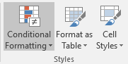
- In the Conditional Formatting options, select “Highlight Cells Rules” and click “More Rules”.

- Now, in the rule description, select “Blanks” from the drop-down menu.

- After that, click on the “Format” button to open the formatting options.

- From formatting options, select the color you want to use for highlighting.
- Click OK.

And the best part is, if you have blank-looking cells with a formula (one that returns “”), it will also highlight them, and if you have a pivot table instead of a normal table, the steps will be the same.
It’s a one-time setup; you don’t have to apply it again and again. Use a table for your data, and conditional formatting will extend when you add new data to the table.
The Blanks rule also treats cells that contain only spaces as blank. If you want to control exactly what counts as blank, use “Use a formula to determine which cells to format” instead, with A1 as the first cell of your selection. The following formula highlights empty cells, cells with “” and cells with only spaces:
=LEN(TRIM(A1))=0
And if you only want truly empty cells (not formulas that return “”), use ISBLANK:
=ISBLANK(A1)
Highlight the Entire Row with a Blank Cell
To highlight the whole row when any cell in it is blank, select the data (say A2:D20) and use the following formula in the rule. The dollar signs lock the columns, so every cell in the row checks the same range:
=COUNTBLANK($A2:$D2)>0
VBA Code to Highlight Blank Cell
I know you have unconditional love for VBA. And, that’s why we have a macro code to apply color to all the blank cells from a selected range.
Sub ColorBlankCells()
Dim rng As Range
Set rng = Selection
rng.SpecialCells(xlCellTypeBlanks).Interior.Color = vbRed
End Sub
When you run this code, it finds all the blank cells in the selected range at once (with SpecialCells) and applies red color to them. If the selection has no blank cells, SpecialCells gives a “No cells were found” error (1004), and like Go To Special, it doesn’t include cells with formulas that return “”.
Read: VBA Tutorial
Conclusion
So these are the three methods that you can use to highlight blank cells. You can use any of these methods that you think is perfect for you. And if you ask me, I always prefer to use conditional formatting because it’s dynamic, so you don’t need to apply it again and again.
I hope these methods will help you in your daily work.
And if you only want to know how many blank cells you have, use COUNTBLANK, like =COUNTBLANK(A1:D20). Note that it counts cells with a formula that returns “” as blank too.
Now tell me one thing. Do you have any other method to apply color to blank cells? Please share it with me in the comment section; I would love to hear from you. And please don’t forget to share this tip with your friends.
Frequently Asked Questions
Why are some blank-looking cells not highlighted?
Go To Special and the VBA code only pick truly empty cells. A cell with a formula that returns “” or a space isn’t empty. Use conditional formatting with =LEN(TRIM(A1))=0 to include those cells.
How do I remove the highlight from blank cells?
For conditional formatting, go to Home ➜ Conditional Formatting ➜ Clear Rules ➜ Clear Rules from Selected Cells. For a fill color applied with Go To Special or VBA, select the cells and choose No Fill.
Can I fill blank cells instead of highlighting them?
Yes. Select the blank cells with Go To Special, type a value like 0, and press Ctrl + Enter. Excel enters that value in all the selected blank cells at once.

I used conditional formatting to point out data entry cells and cells with formulas.
On all spreadsheets I use:
Formula:=ISBLANK($A$1:$F$5) as rule 1 highlighted light yellow
and
Formula:=ISFORMULA($A$!:$F$5) as rule 2 highlighted light green
The yellow cells reminds me to enter data and the green cells not to change.
I liked very much
One more way that sometimes helps me: I take a sharpie and mark them on the screen. I usually use my right most screen because I don’t use it as much as the other two and the sharpie will look silly if the Excel spreadsheet is not up. Note: this is not a dynamic solution. It is very much a static fix.
I don’t have another way, but would like to say that conditional formatting would be the only way I’d do it. Only downside is Excel does corrupt it’s conditional formatting from time to time so you may need to repair them, which means you need to document what they are, why, etc so you can reset them when that happens.
Manually highlighting the cells would be okay in a one-off spreadsheet (because values won’t really change), but would look odd when later on a value appeared!
I avoid VBA as much as possible, hence I don’t have a personal library available to any & every XLSX I create – others would be unlikely to have the same so the spreadsheet wouldn’t work for them. Also just like using “Goto Special”, the VBA is also a one-time event. The user would need to then rerun the macro to update the highlighting.
Last point – the VBA should be enhanced to revert the colour back to default if it not blank so it would not remain highlighted if the cell now has a value.
I had not seen the Conditional Formatting “Format only cells that contain” option BLANK … Thanks, my lesson for today!.
I use Conditional Formatting “Use a formula to determine which cells to format” with =isBlank () and =isFormula () to shade blank cells yellow and cells with formulas light green. Keeps me from missing something and messing up equations.
Thanks, as always; a fantastic support.