

Select the cell and press Ctrl + K, or right-click and choose Link. In the Insert Hyperlink dialog, pick Existing File or Web Page and paste a URL into Address, or pick Place in This Document to jump to a sheet and cell in the same workbook. Type the label you want in Text to display and click OK.
To link to a particular cell in another workbook, choose Existing File or Web Page, select the file, then click Bookmark to pick the sheet and cell. For an email link, choose E-mail Address and fill in the address and subject.
To build links with a formula, use =HYPERLINK("https://excelchamps.com","ExcelChamps") for a web page, =HYPERLINK("#Sheet2!A1","Go to Sheet2") for a cell in the same workbook, and =HYPERLINK("mailto:name@example.com","Email us") for email. The # keeps the link inside the workbook; wrap a sheet name with spaces in single quotes, as in "#'Sales Data'!A1".
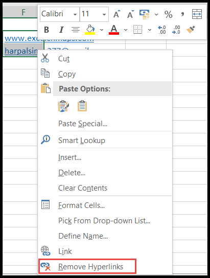
To remove a link, right-click the cell and choose Remove Hyperlink. For many cells, select them (or press Ctrl + A for the whole sheet) and go to Home → Clear → Remove Hyperlinks, which also strips the blue underline, or Home → Clear → Clear Hyperlinks to keep the formatting.
Two things catch people out. Links made with the HYPERLINK function are formulas, so Remove Hyperlink leaves them working; copy those cells and paste them as values to keep the text without the link. And if Excel keeps turning typed URLs and email addresses into links, press Ctrl + Z straight after typing to undo that one, or turn it off under File → Options → Proofing → AutoCorrect Options → AutoFormat As You Type by clearing Internet and network paths with hyperlinks.
A hyperlink in Excel is a link to a specific file, document, location, web page, or email address. By using a hyperlink, users can go to a specific file, document, or location.
By adding a web or email address to the hyperlink, users can navigate to a web page or send an email to a specified email address just by clicking on that link.
Hyperlinks are easy to recognize, as they are underlined blue or purple text. We have mentioned some quick and easy steps for you to add and remove hyperlinks in Excel.
Add Hyperlink to an Existing Workbook
Adding hyperlinks in Excel is very easy and quick. Users can add hyperlinks manually to Excel. Excel also automatically creates a hyperlink when users enter any web address or email address in a cell.
- First, go to the “Insert” tab and then click on the “Link” icon in the “Links” group.

- Or, right-click on the cell where you want to add the hyperlink, and then click on the “Link” option from the pop-up menu.
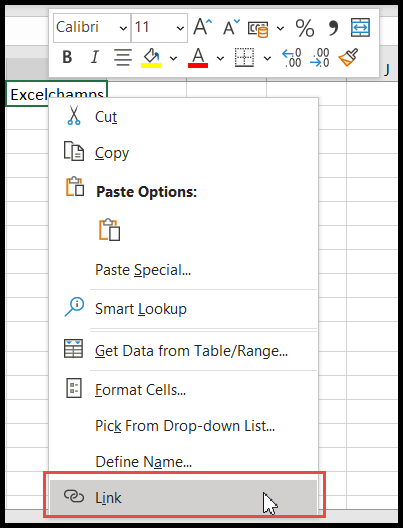
- Or, press the CTRL + K shortcut on the keyboard.
- Once you follow any of the above steps, the “Insert Hyperlink” window opens.
- After that, select the “Existing File or Web Page” option and then select the location where that file or document is placed.
- Now, select the file or document and then enter the text in the “Text to display” box which you want to display as a hyperlinked name, and click OK.
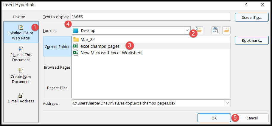
Add Hyperlink to a Specific Sheet of an Existing Workbook
- First, select the “Existing File or Web Page” option and then select the location where that file or document is placed.
- After that, select the file or document and then click on the “Bookmark” button.
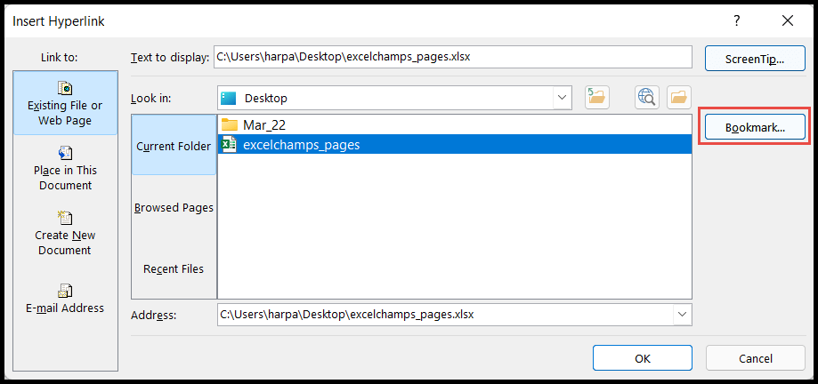
- Now, select the specific sheet and the targeted cell of that existing sheet and click OK.
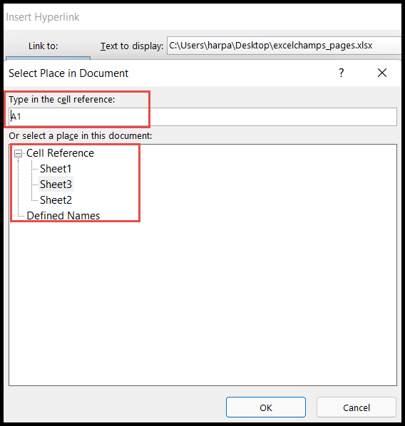
Add Hyperlink to a Specific Sheet of the Current Workbook
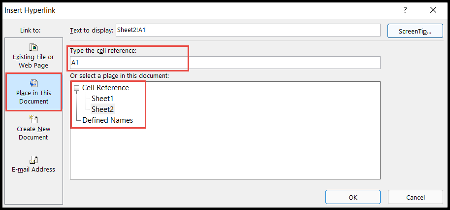
- First, select the “Place in This Document” option, and you will get all the sheets of the current workbook.
- After that, select the specific sheet and the targeted cell and click OK.
Add Hyperlink to a Web Address
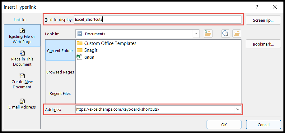
- First, open the web page in the browser and copy the web address and paste it into the “Address” box in the “Insert Hyperlink” window.
- After that, enter the text in the “Text to display” box that you want to display as a hyperlinked name, and then click OK.
Add Hyperlink to Open a New Workbook
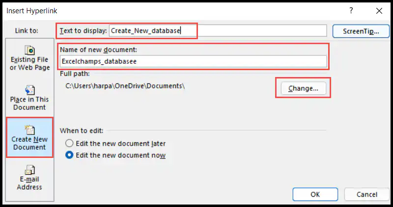
- First, select the “Create New Document” option and enter the name of the new workbook in the “Name of new document” box.
- After that, enter the text in the “Text to display” box that you want to display as a hyperlinked name.
- Now, click on the Change button if you want to change the saving location of the new workbook, and click OK.
Add Hyperlink to an Email Address
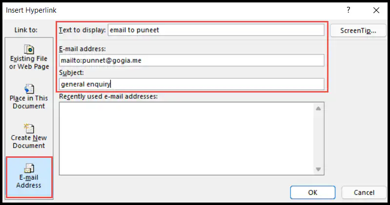
- First, select the “E-mail Address” option and then enter the email address in the “E-mail address:” box and enter the email subject in the “Subject” box.
- After that, enter the text in “Text to display” which you want to display as a hyperlinked name, and click OK.
- You can even directly enter the email address in the cell and Excel will auto-create the hyperlink to that email.
Remove Hyperlinks in Excel
Removing hyperlinks from Excel is way easier and quicker than adding or creating hyperlinks. Excel allows users to remove hyperlinks in just two clicks, as mentioned below.
- To remove a hyperlink from a cell, right-click on a cell containing a hyperlink and then click on “Remove Hyperlink” from the pop-up menu.

- To remove hyperlinks from multiple cells, select the cells together, right-click, and select “Remove Hyperlinks” from the pop-up menu.
- To remove all the hyperlinks from the current worksheet, select the whole worksheet by pressing CTRL+A (press it twice if the active cell is inside a data range).
- Now, go to the “Home” tab, click on the “Clear” drop-down arrow in the Editing group, and then select “Remove Hyperlinks”.
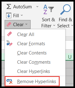
In the same Clear menu, you also have “Clear Hyperlinks”. It removes the link but keeps the blue underlined format, while “Remove Hyperlinks” removes both the link and the formatting.
Add a Hyperlink with the HYPERLINK Function
You can also create a link with a formula. The HYPERLINK function takes the address and the text to show, so the link can change with the values in your cells:
=HYPERLINK("https://excelchamps.com","Visit ExcelChamps")
To link to a cell in the same workbook, start the address with a # sign:
=HYPERLINK("#Sheet2!A1","Go to Sheet2")
Edit or Select a Cell with a Hyperlink
To change a link, right-click the cell and click “Edit Hyperlink”, or select the cell and press Ctrl + K. And to select a cell with a hyperlink without opening the link, click the cell and hold the mouse button until the pointer changes to a plus sign, or select a cell next to it and use the arrow keys.
Stop Excel from Creating Hyperlinks Automatically
If you don’t want Excel to turn web and email addresses into links, go to File ➜ Options ➜ Proofing ➜ AutoCorrect Options ➜ AutoFormat As You Type, and untick “Internet and network paths with hyperlinks”. To undo a single automatic link right after you type it, press Ctrl + Z.
Remove All Hyperlinks with VBA
The following code removes all the hyperlinks from the active sheet in one go (links created with the HYPERLINK function are formulas, so they stay):
Sub remove_all_hyperlinks()
    ActiveSheet.Hyperlinks.Delete
End Sub
Frequently Asked Questions
Why is my hyperlink not working?
The file has been moved or renamed, the sheet name in the link has changed, or the web address is wrong. Right-click the cell, choose Edit Hyperlink, and fix the address.
Why doesn’t Remove Hyperlinks remove my HYPERLINK formulas?
Because those links come from a formula, not from the Insert Hyperlink option. Delete the formula, or convert it to a value (Copy ➜ Paste Values) to keep only the text.
Can I link to a named range?
Yes. In Place in This Document, the Defined Names list shows the named ranges of the workbook. Select one and click OK.