Excel Wildcard Characters: Types and Usage

What are Excel Wildcard Characters

Excel wildcard characters are placeholders that stand in for characters you don’t know. Instead of matching a value exactly, you supply the part you’re sure about and let the wildcard cover the rest, so Pi* finds Pivot, Picture, and Picnic in one go. Excel supports three, and they work in criteria arguments, lookups, filters, and Find and Replace.

Types of Excel Wildcard Characters

Excel has three wildcard characters: the asterisk (*), the question mark (?), and the tilde (~). The first two stand in for unknown characters: the asterisk for any number of them, the question mark for exactly one. The tilde does the opposite job: it cancels a wildcard, so Excel treats it as a literal character.

1. Asterisk(*)

The asterisk is the most-used wildcard. It stands in for any number of characters, zero, one, or fifty. So Pi* returns Pivot, Picture, and Picnic, because everything after Pi is left open. Move it to the front (*ing), and you match endings instead; put one on both sides (and) and you match the text anywhere in the cell.

To count the cities in each classification, a plain COUNTIF won’t work; the classification shares a cell with the city name. An asterisk covers the rest.

=COUNTIF(City,Tier-2&"*")

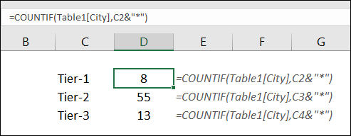
Here, the & joins the classification text from the cell to an asterisk, so the criteria becomes something like Metro*. Because the asterisk sits at the end, COUNTIF matches every entry that starts with that classification, no matter what follows it. That gives you the count of cities in each classification without having to split the column first.

2. Question Mark

A question mark stands in for exactly one character. It’s the precise option — use it when you know how many characters are missing, not just that something is missing. For example, ch?mps returns both champs and chimps, because the ? accepts any single character in that one position. ??amps would work the same way for two unknown characters.

3. Tilde (~)

The real use of a tilde is to nullify the effect of a wildcard character. For example, let’s say you want to find the exact phrase pivot*. If you use pivot* as a string, it will give you any word that has pivot at the beginning (such as pivot table or pivot chart).

To find the text pivot*, put a tilde directly before the asterisk: pivot~. The tilde tells Excel to treat the very next character as ordinary text rather than a wildcard, so this matches only the exact string pivot — not pivot table or pivot chart. The same trick works for a literal question mark (~?) and for a literal tilde itself (~~).

Wildcard Characters with Excel Functions

We can easily use all three wildcard characters with all the top functions. Functions like VLOOKUP, HLOOKUP, SUMIF, SUMIFS, COUNTIF, COUNTIFS, SEARCH, FIND, and Reverse LOOKUP.

You can extend this list with all the functions that you use for matching a value, for lookups, or for finding text. Ahead, I’ll share with you some examples with functions + find and replace options + conditional formatting + numbers.

1. With SUMIF

Below is a list of invoice numbers with their amounts. Each invoice number starts with a product code, so to total the sales for Product-A, you need to sum every row whose invoice number begins with Product-A. This is where the asterisk comes in. It stands for “anything at all”, so “Product-A*” tells Excel to match the text Product-A followed by whatever comes after it.

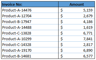
To do this, we can use SUMIF with wildcard characters. The formula will be:

=SUMIF(F2:F11,"Product-A*",G2:G11)

The asterisk sits at the end of the criteria, so SUMIF matches any invoice number that begins with “Product-A” and ignores whatever follows. Move it to the front (“*Product-A”) and you’d match values ending with it instead.

2. With VLOOKUP

Let’s say you have a list of students with full name and their marks. Now, you want to use VLOOKUP to get marks in another list in which you only have their first names.

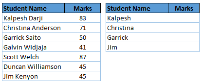
For this, the formula will be:

=VLOOKUP(first_name&”*”,marks_table,2,0)

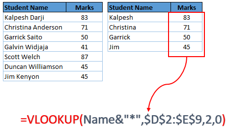
In the example above, you used VLOOKUP with an asterisk to get marks using only the first name.

3. For Find and Replace

Using wildcard characters with the Find and Replace option can do wonders for your data.

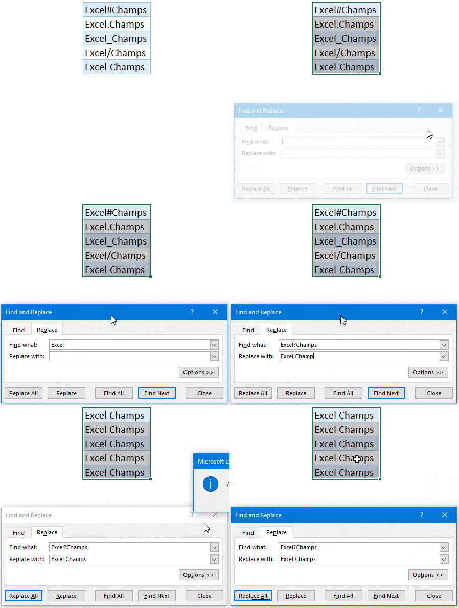
In the data below, “Excel” and “Champs” are separated by a different character in each row. Replacing them one by one would take as many passes as there are characters; instead, find Excel?Champs and replace it with Excel Champs. The question mark matches whatever single character sits in that position, so every variation gets cleaned in one go.

4. In Conditional Formatting

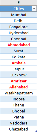
You can also use these wildcard characters with conditional formatting. Let’s say, from a list, you want to highlight the names of the cities that start with the letter A.

• First of all, select the first entry from the list and then go to Home → Styles → Conditional Formatting.
• Now, click on the “New Rule” option, and select use a formula to determine which cells to format”.
• In the formula input box, enter =IF(COUNTIF(E2,"A*"),TRUE,FALSE).
• Set the desired formatting you want to use to highlight.

• Now, I have used conditional formatting in the first cell of the list & I have to apply it to the entire list.
• Select the first cell on which you have applied your formatting rule.
• Go to Home → Clipboard → Format Painter.
• Select the entire list, and it will highlight all the names starting with the letter A.

5. Filter values

Wildcards also work in Excel’s filter dropdowns. Say you have a list of cities and you want to see only the ones starting with A, type A* into the filter’s search box and Excel shows just those. Swap the letter for any other, or use *A to match names ending in A instead.

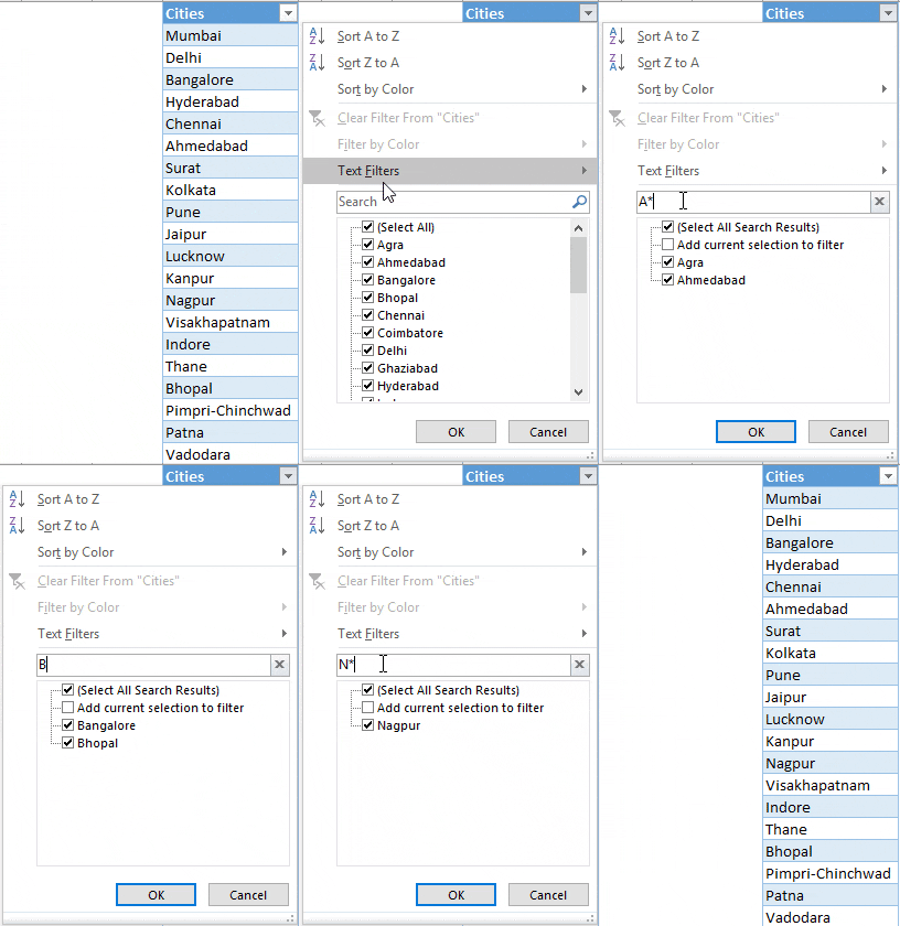
This will give you the exact name of cities that are starting from that letter. And, if you want to search for any character which is ending with a specific letter you can use it before that letter (*A, *B,*C, etc.).

6. With Numbers

You can use these wildcards with numbers but you have to convert those numbers into text.

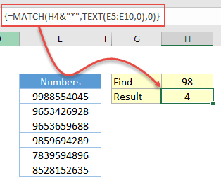
In the above example, you have used the match function and text function to perform a partial match. The text function returns an array by converting the entire range into the text and after that match function, lookup for a value starting from 98.

Sample File

Download this sample file from here to learn more.

Conclusion

With wildcard characters, you can enhance the power of functions when your data is not in a proper format. These characters help you search or match a value using a partial match which gives you the power to deal with irregular text values. The best part is that you have three different characters to use.

Have you ever used these wildcard characters before?

Share your views in the comments; I’d love to hear from you. And don’t forget to share this tip with your friends.