In Excel, columns have alphabets as their identity, but you can change it to a number. That means for column A you can use column 1. In this tutorial, we will learn two different ways that you can use.
- Create Header Row with Column Number
- Change Cell Reference to R1C1 to Apply for Column Numbers

Change Column Alphabets to Number (R1C1)
- First, click on the File Tab.

- After that, go to “Options”.

- Next, click on the “Formulas” and from there, tick mark the “R1C1 reference style”.

- In the end, click OK to apply the settings.

When you do this, it changes the reference style for the entire Excel application. That means now you need need to refer to a column using a number, not by the alphabet.
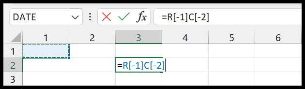
You see in the above example where I am referring to cell A1 it shows R[-1]C[-2] instead of the A1. Well, this means you are referring to the one row and two columns backward.
You can learn more about it from this complete guide on the R1C1 reference style.
Create a Header with Column Numbers
This method could be used in different situations, but as effective as the first one.
- First, edit cell A1 and enter “=COLUMN()” in it.

- After that, hit enter to get the number of the current column.

- Now, use the fill handle and extend the formula to the column you want to have column numbers.

- In the end, you can convert all these formulas into values by using the keyboard shortcut (Ctrl + C to copy and then press Alt → H → V → V to paste the values).
This method works better when you don’t want to change the cell reference but want column number only.