How to Rename a Table in Excel

Why there is a Need to Rename a Table

If you’ve ever found yourself lost in a sea of ‘Table1’, ‘Table2’, and so on, you know the immense value that intelligently named tables can bring to your Excel workflow.

When applying an Excel table to a data set, Excel allows you to name it. But by default, a generic name is given to a table.

In this comprehensive guide, we’ll dive into renaming a table in Excel.

We’ll explain each step in detail and even show you how to use Excel’s Name Manager and keyboard shortcuts to rename tables more efficiently.

But, in this tutorial, we will learn quick steps to rename a table with a custom name.

Change the Name of an Excel Table (Existing Table)

Please note that table names in Excel must be unique within a workbook.

Here’s a step-by-step guide on renaming a table in Excel:

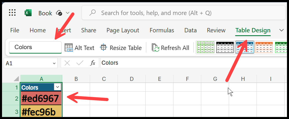
1. Select the Table – First, click anywhere within the table you want to rename. After you click on the table, a new tab labeled ‘Table Design’ appears on the Excel ribbon at the top of the window.
2. Access Table Design – Next, click on the ‘Table Design’ tab to open it. This tab provides various options for changing tables. It’s split into several groups, each containing relevant commands.
3. Go to the Properties Group – Locate the’ Properties’ group within the ‘Table Tools’ tab. This group contains options related to your table’s properties.
4. Rename the Table – The current name of the table is displayed in the ‘Table Name’ field inside the’ Properties’ group. To rename the table, click in the ‘Table Name’ field, delete the existing name, and type the new name you want to use.
5. Save the New Table Name – After typing the new name, press Enter to save it. Your table now has a new, more descriptive name.

Alert: You can’t just delete a table’s name; you need to specify a new name.

Use Name Manager to Rename an Excel Table

This method is amazing if you want to rename more than one table.

1. First, go to the Formulas Tab and click on the “Name Manager” option.
   
2. From there, select the table you want to rename and click edit.
   
3. Now, from the name input bar, change the name.
   
4. In the end, click OK to save, and then click on Close.
   

Tip: By using name manager, you can manage all tables that you have in a workbook.

Keyboard Shortcut to Change the Name of a Table

To rename a table in Excel using a keyboard shortcut, use the below shortcut:

ALT > J + T > A

• Select any of the cells within the table.
• Press Alt, J, T, and A in sequence (not simultaneously) to open the ‘Table Name’ field in the ‘Table Design’ tab.
• Type the new name and press Enter.

Rename a Table in Excel for the Web

Renaming a table in Excel for the web is a straightforward process. Here is a detailed step-by-step guide on how to do it:

1. Select the Table: To rename a table, click anywhere within it. This action will select the entire table.
2. Go to the Table Design: Look at the Excel ribbon at the top of your screen. Navigate to the “Table Design” tab on the Excel ribbon. This tab is specifically designed to handle all table style and other options.
3. Rename the Table: You will see a “Table Name” field (first from the left side). This field displays the current name of your table. Click in the “Table Name” field, which will allow you to modify the table’s name. The existing name will become highlighted or have a cursor at the end, indicating you can start typing to replace it. Delete the existing name and type your new name for your table.
4. Save the New Table Name: Press the Enter key on your keyboard after typing the new name. This action will save the new name for your table. The new name will immediately appear in the “Table Name” field, indicating the change has been successfully applied.

Notes on Naming Tables

1. The name of a table needs to be a hard code value. You can’t refer to a cell for the name.
2. You can’t use a space in between the name of the table. But you can use a hyphen or underscore to make it readable.
3. You must start the name with a letter, underscore (_), or backslash (/).
4. The length of the name can be up to 255 characters, but you hardly need to use a name that long.
5. The name of each table in a workbook needs to be unique (if you have multiple tables).

Renaming a Table in Excel with a Meaningful Name

• Improves Clarity: Using a meaningful name can make identifying the table’s data easier.
• Simplifies Navigation: If you have two or three tables in a workbook, naming them can make it easier to navigate between them.
• Enhances Formula Readability: When using table data in formulas, Excel automatically uses structured referencing, which includes the table name. This can make formulas more straightforward to read and understand.
• Promotes Consistency: Using a consistent naming convention can make your workbook more organized and easier to manage if you work with more than one table.