

To grey out cells based on a condition, select the range (say A2:F100), go to Home → Conditional Formatting → New Rule → Use a formula to determine which cells to format, enter a formula such as =$F2="Closed", and choose a grey fill and grey font under Format.
To grey out every empty cell, click the Select All corner above row 1 and use =A1="" in the same kind of rule. Pressing Ctrl + A once inside your data selects only the data block, so press it twice or use the corner button.
To show only the area you use, hide everything around it. Click the header of the first empty column, press Ctrl + Shift + →, right-click and choose Hide. Do the same for rows with Ctrl + Shift + ↓. The space beyond your data then shows as plain grey.
For a quick view that changes nothing, use View → Page Break Preview. Cells outside the print area turn grey, so set the print area first with Page Layout → Print Area → Set Print Area.
Greyed-out cells can still be edited. To stop people typing in them, unlock the cells they should use (Ctrl + 1 → Protection, untick Locked), then turn on Review → Protect Sheet.
When you are sharing a report or data with someone, you can grey out all the unused cells. That helps the user stay focused only on the part of the worksheet where you have data.
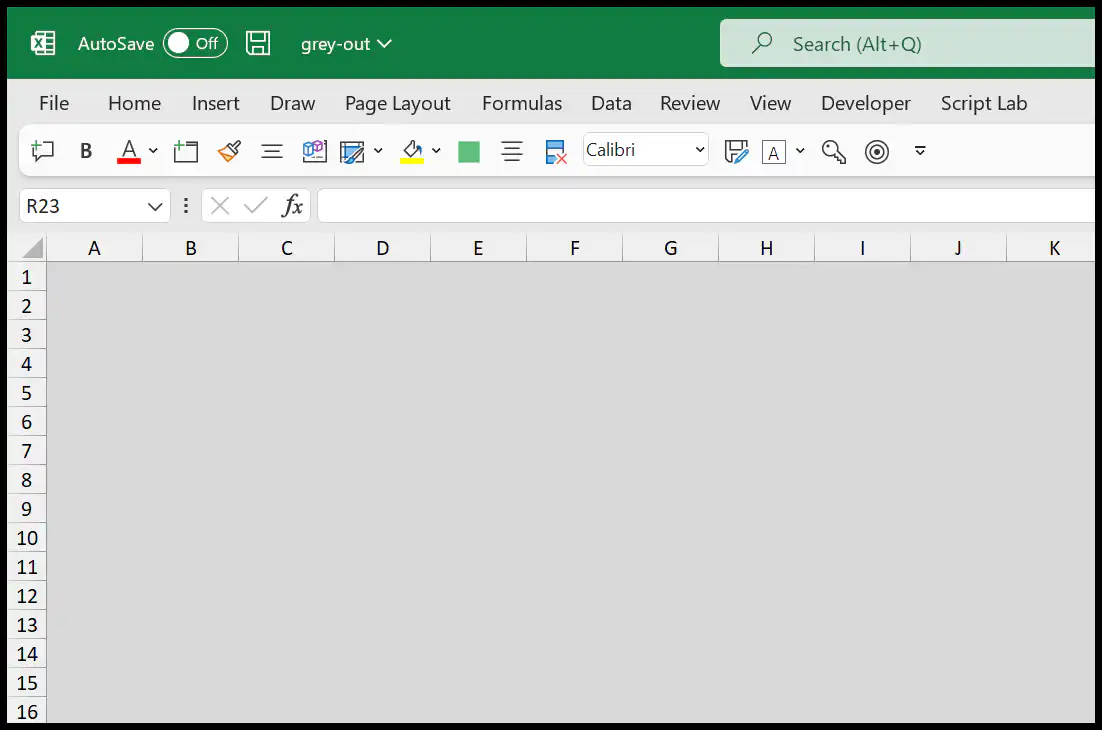
In this tutorial, we will look at a few different ways to add grey color to the cells which are not used.
Use Conditional Formatting to Grey Out Unused Cells
- First, select cell A1 and use the keyboard shortcut Ctrl + A to select all the cells.
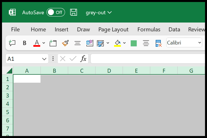
- Now, go to the Home tab, click on Conditional Formatting, and then select the New Rule option.
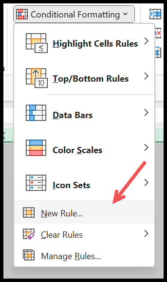
- After that, in the New Formatting Rule dialog box, click on “Use a formula to determine which cells to format”.
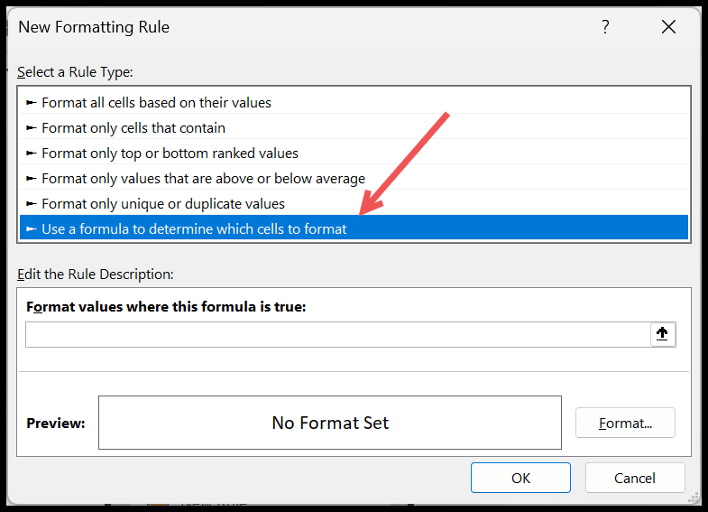
- From here, in “Format values where this formula is true”, enter the formula (shown below this list).

- Next, click on the “Format” button, go to the Fill tab, and select the grey color.
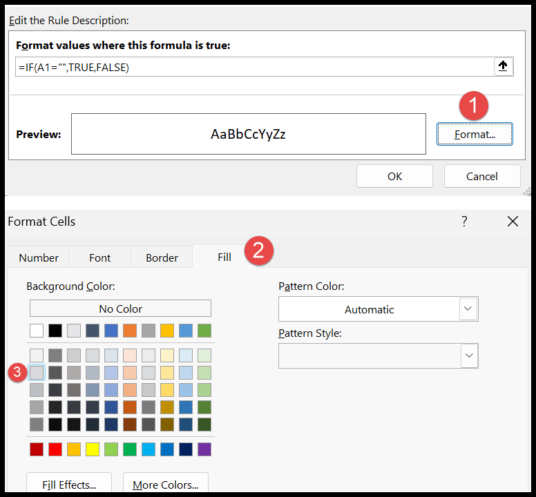
- Click OK to save the rule.
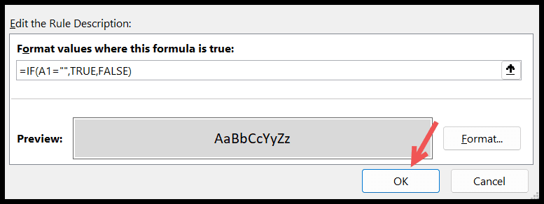
Here’s the formula for step 4:
=IF(A1="",TRUE,FALSE)
As the formula itself returns TRUE or FALSE, you can also use the shorter version below. Both work the same way. Make sure A1 has no dollar signs, so the rule moves with each cell.
=A1=""
It greys all the empty cells in your worksheet, and the moment you enter a value in a cell, the grey fill goes away automatically.
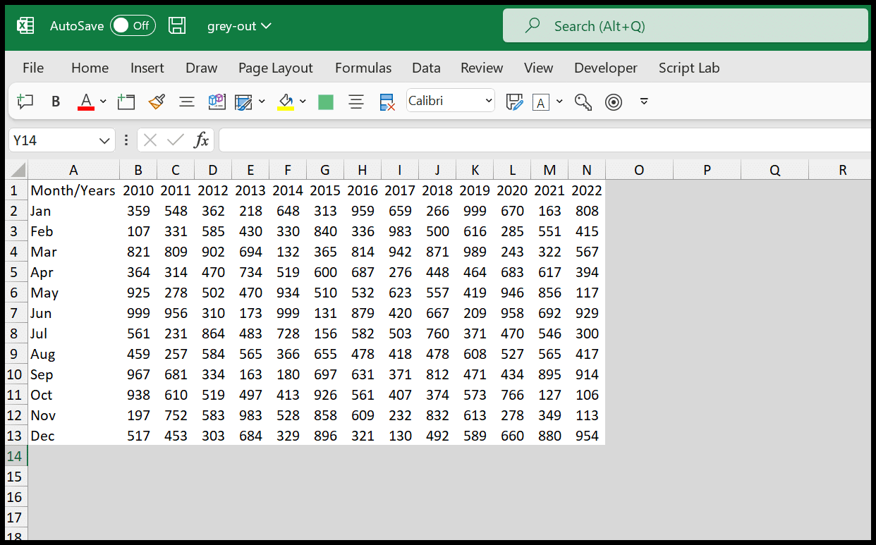
Keep in mind that this rule also greys the empty cells inside your data, and cells with a formula that returns count as empty too. A cell with only a space is not empty, so it stays white.
Quick Read: How to Print Specific Cells in Excel
Hide Rows and Columns to Grey Out Unused Areas
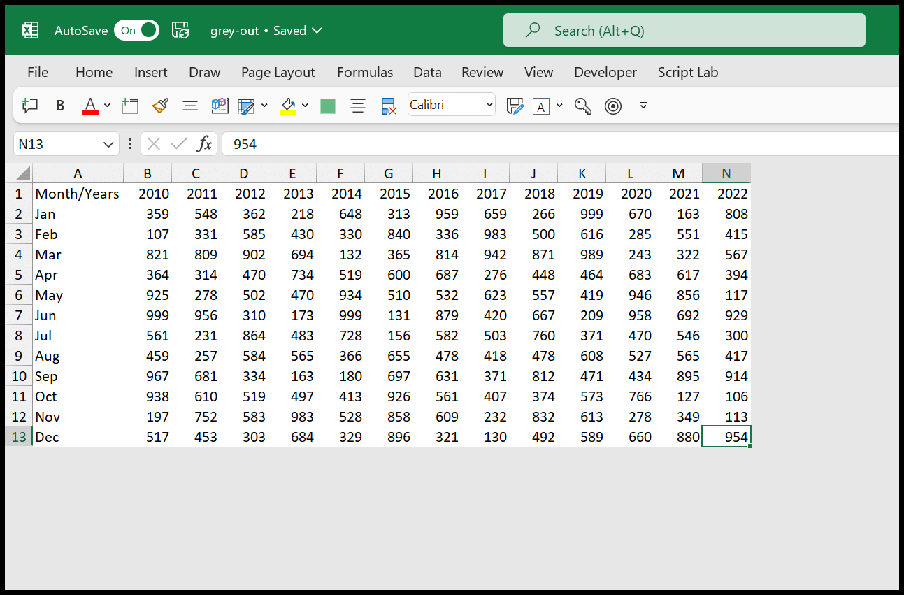
Apart from the above method, you can simply hide all sections of the worksheet where you don’t have any data. In the following example, you have data from cells A1 to N13.
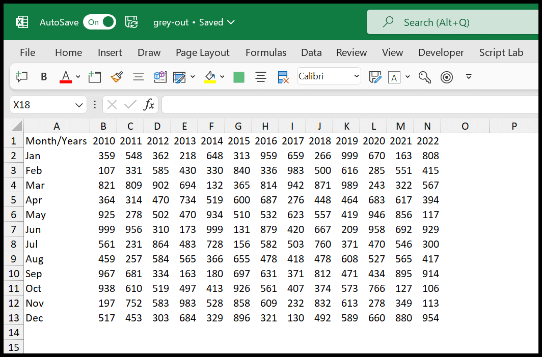
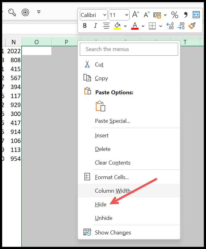
Select all the columns after column N (click the header of column O and press Ctrl + Shift + Right Arrow), right-click, and click on the Hide option.
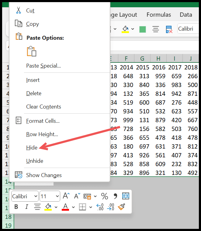
Now select all the rows after row 13 (click the header of row 14 and press Ctrl + Shift + Down Arrow), right-click, and select the Hide option from there.
The moment you do this, all the rows below row 13 will be hidden, and all the areas where you don’t have data are greyed out. To get them back, select the whole sheet (Ctrl + A), right-click a column header and click Unhide, and do the same for the rows.
Use Page Break View to Grey Out Cells
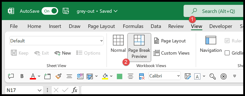
If you don’t want to change anything in your worksheet, you can use Page Break Preview, which shows all the unused cells greyed out.
Go to the View Tab → Workbook Views → Page Break Preview.
After that, you need to change the zoom level to 100% because when switching to Page Break Preview, Excel changes the zoom level to 60%.
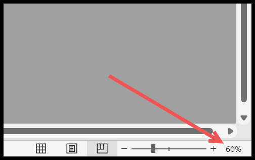
Change the zoom level to 100%, and you will have a worksheet view just like the following.
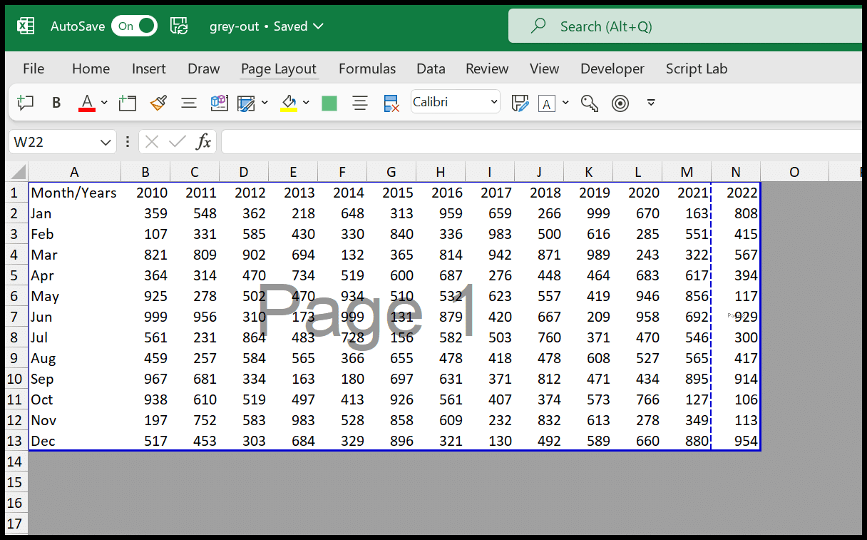
Page Break Preview shows the print area in white and everything else in grey. If you have set a print area, only that area stays white. To go back, click View ➜ Normal.
Frequently Asked Questions
Does greying out cells affect printing?
Conditional formatting prints the grey fill if the cells are in the print area, while hidden rows and columns and Page Break Preview don’t print anything extra. Set a print area if you only want to print your data.
How do I remove the grey from all the cells?
For the conditional formatting method, go to Home ➜ Conditional Formatting ➜ Clear Rules ➜ Clear Rules from Entire Sheet. For hidden rows and columns, select the sheet and unhide them, and for Page Break Preview, switch back to Normal view.
Can I stop users from scrolling to the grey area?
Yes. Hiding the unused rows and columns does that, as there’s nothing left to scroll to. If you also protect the sheet, users can’t unhide them.