Sum IF Cell Contains a Specific Text (SUMIF Partial Text)

To sum values from cells where you have a specific text or a partial text, you need to use wildcard characters with SUMIF.

In the criteria argument, you need to use an asterisk before and after the text using an ampersand, just like we have used in the following example to sum cells where you have the text “Mobile” in the “Product” column.

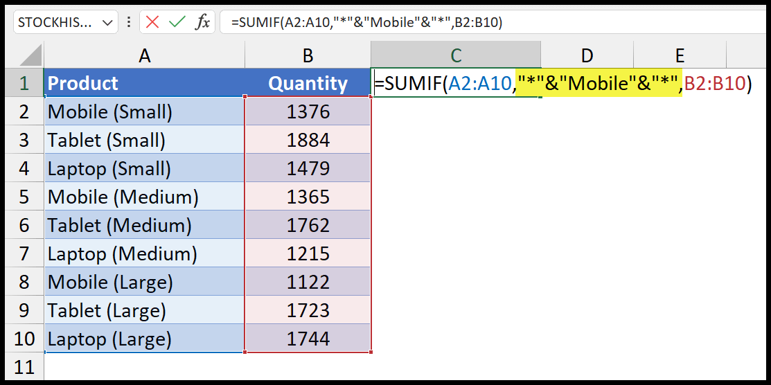
In this tutorial, we will learn to write this formula by using SUMIF.

Formula to Sum IF Cell Contains a Specific Text

1. First, in cell C1, enter “=SUMIF(“.
2. After that, refer to the range from which we need to check the criteria.
3. Now, in the criteria, enter an asterisk-criteria-asterisk (“*”&”Mobile”&”*”).
4. Next, in the sum_range argument, refer to the quantity column.
5. In the end, hit enter to get the result.

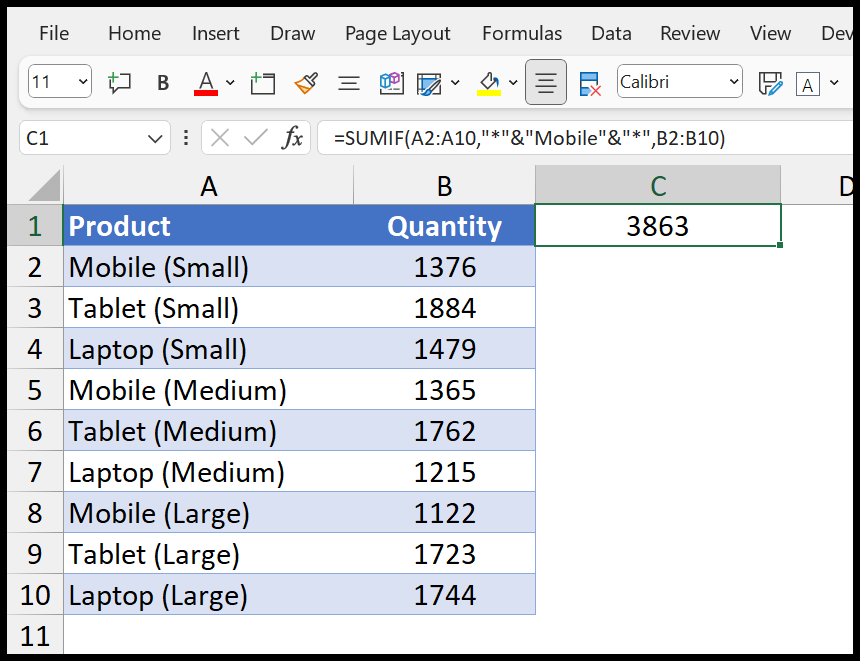
=SUMIF(A2:A10,"*"&"Mobile"&"*",B2:B10)

The formula looks at each cell in the range A2 through A10 and checks if the word “Mobile” appears anywhere in each of these cells.

The “*” wildcard character on both sides of “Mobile” tells Excel to ignore what comes before or after it, which makes it a partial text.

And apart from this, SUMIFS can be used if you have multiple conditions.

=SUMIFS(sum_range, criteria_range1, "*text*")

SUM IF Cell Contains Partial Text using Case-Sensitive

If you want to sum values based on a case-sensitive search, use an array formula combining FIND, IF, and SUM. This formula allows for a manual array setup to handle case-sensitive partial text match.

=SUM(IF(ISNUMBER(FIND("MOBILE", A2:A10)), B2:B10, 0))

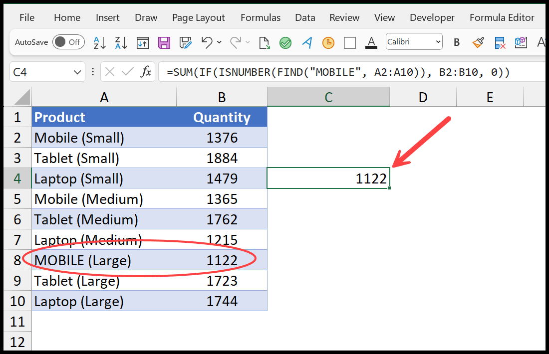
Note – For this formula to work as an array formula in some versions of Excel, you need to enter it with Ctrl+Shift+Enter.

This formula sums values from column B, but only for column A rows containing the exact word “MOBILE” with the same uppercase letters.

Here’s how it works: The formula goes through each cell in the range A2 to A10 and uses the FIND function, which is case-sensitive, to look for the value “MOBILE”.

If “MOBILE” is found, FIND returns a number indicating where “MOBILE” starts in the text. The ISNUMBER function checks if FIND returned a number (meaning “MOBILE” was found). If it did find “MOBILE”, the corresponding value from column B is included in the sum.

If “MOBILE” wasn’t found, or if it’s in a different case (like “Mobile” or “mobile”), it adds zero instead for that row. This way, the formula only adds up the numbers from column B where “MOBILE” exactly matches in column A.

Use Dynamic Functions to Sum Values on a Partial Text

Yes, you can utilize Excel’s dynamic array functions to sum if a partial text matches more dynamically and efficiently, especially with newer versions of Excel that support these features.

Let’s say, column A contains product names, and column B contains corresponding sales figures. You want to sum all sales values where the product name contains “Mobile”:

=SUM(FILTER(B:B, ISNUMBER(SEARCH("Mobile", A:A))))

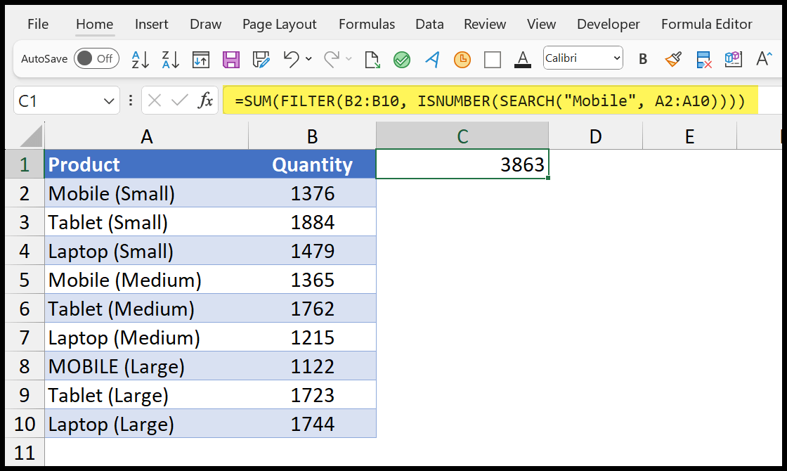
This formula sums up values from column B, but only for rows where the word “Mobile” is found in column A.

It searches for “Mobile” in each cell of column A and, if found, adds the corresponding value from column B in the total. If “Mobile” isn’t found in any cell, or if there’s an error, the formula returns 0.

But if no cells meet the criteria, FILTER will show an error, which you can handle with IFERROR:

=IFERROR(SUM(FILTER(B:B, ISNUMBER(SEARCH("Mobile", A:A)))),0)

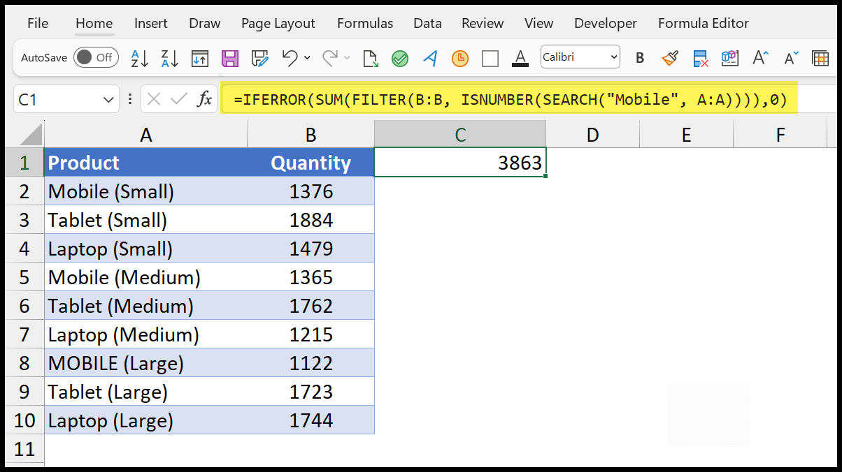
Or you can also go with BYROW in combination with SEARCH.

=SUM(BYROW(A:A, LAMBDA(cell, IF(ISNUMBER(SEARCH("Mobile", cell)), INDEX(B:B, ROW(cell)), 0))))

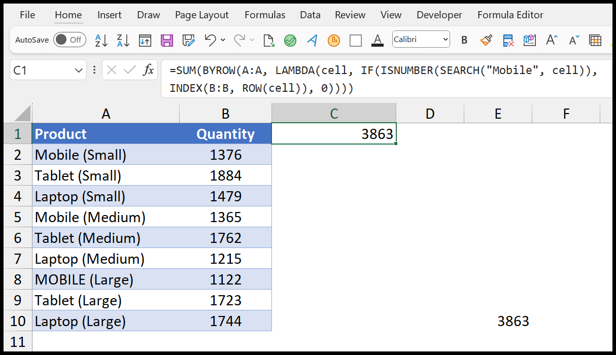
This formula goes through column A’s row to check if it contains the word “Mobile”. If the word “Mobile” is found in a row, the formula looks at the corresponding row in column B and takes that sales value.

If the text “Mobile” is not found, it takes zero instead. Add up all the numbers that were picked from column B.

Use a Custom Function to SUM Values Based on a Partial Text

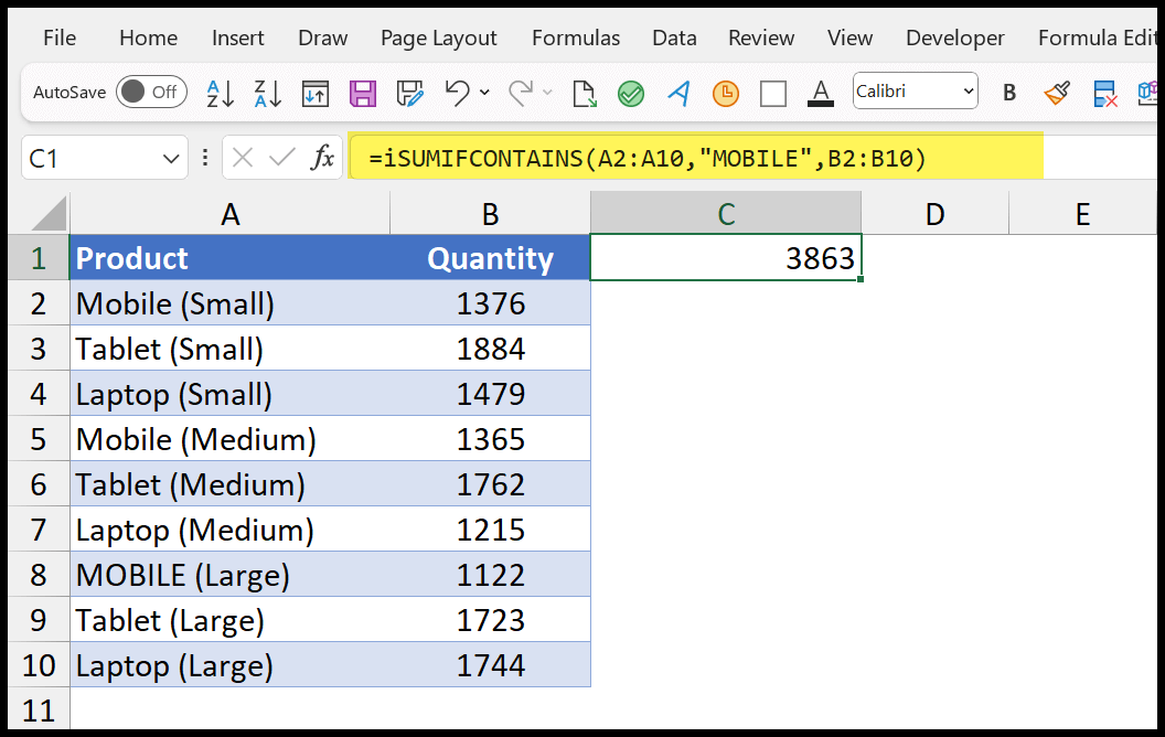
And if you like to use a custom function for this well, here’s a VBA function that performs a case-insensitive sum based on a partial text match:

Function iSUMIFCONTAINS(searchRange As Range, searchText As String, sumRange As Range) As Double
    Dim cell As Range
    Dim sumResult As Double
    
    ' Initialize the result variable.
    sumResult = 0
    
    ' Check if both ranges are of the same size
    If searchRange.Rows.Count <> sumRange.Rows.Count Or searchRange.Columns.Count <> sumRange.Columns.Count Then
        iSUMIFCONTAINS = CVErr(xlErrRef)
        Exit Function
    End If
    
    ' Loop through all cells in the searchRange
    For Each cell In searchRange
        If InStr(1, cell.Value, searchText, vbTextCompare) > 0 Then
            ' If searchText is found, add the corresponding value from sumRange
            sumResult = sumResult + sumRange.Cells(cell.Row - searchRange.Row + 1, cell.Column - searchRange.Column + 1).Value
        End If
    Next cell
    
    ' Return the result
    iSUMIFCONTAINS = sumResult
End Function

=iSUMIFCONTAINS(A2:A10,"Mobile",B2:B10)

Function iSUMIFCONTAINS(searchRange As Range, searchText As String, sumRange As Range, Optional caseSensitive As Boolean = False) As Double
    Dim cell As Range
    Dim sumResult As Double
    Dim compareMode As Integer
    
    ' Determine comparison mode based on case sensitivity option
    If caseSensitive Then
        compareMode = vbBinaryCompare ' Case-sensitive
    Else
        compareMode = vbTextCompare  ' Case-insensitive
    End If
    
    ' Initialize the result variable.
    sumResult = 0
    
    ' Check if both ranges are of the same size
    If searchRange.Rows.Count <> sumRange.Rows.Count Or searchRange.Columns.Count <> sumRange.Columns.Count Then
        iSUMIFCONTAINS = CVErr(xlErrRef)
        Exit Function
    End If
    
    ' Loop through all cells in the searchRange
    For Each cell In searchRange
        If InStr(1, cell.Value, searchText, compareMode) > 0 Then
            ' If searchText is found, add the corresponding value from sumRange
            sumResult = sumResult + sumRange.Cells(cell.Row - searchRange.Row + 1, cell.Column - searchRange.Column + 1).Value
        End If
    Next cell
    
    ' Return the result
    iSUMIFCONTAINS = sumResult
End Function

=iSUMIFCONTAINS(A2:A10,"MOBILE",B2:B10,TRUE)