Sum Values Based on Year (SUMIF Year)

To sum values, based on a specific year, in Excel, we gave two methods to follow. The first method uses a helper column where you need to add a column with the year number and sum values based on the month from that column.

The second method uses a different approach. To create an array by extracting months from the date column and then sum values based on a year from that array.

In this tutorial, we will learn both methods to sum values based on a year.

SUMIF Year with a Helper Column

1. First, add a new column and enter the YEAR function to get the year number from the dates.
   
2. Now, go to the next column and enter the SUMIFS function there.
3. In the SUMIF function, refer to the year column for the range argument.
   
4. Next, in the criteria argument, enter the year that you want to use to sum values.
   
5. In the end, refer to the quantity column for the sum_range, enter the closing parentheses, and hit enter to get the result.
   

Once you hit enter, there with the sum values for the year 2021, as you have mentioned in the criteria.

=SUMIF(C1:C16,2021,B1:B16)

Use SUMPRODUCT to Sum Values Based on a Year

Creating a formula by using SUMPRODUCT is way more powerful. With this formula, you don’t need to add a helper column.

1. First, enter the SUMPRODUCT function and enter the double minus sign “–“.
2. After that, enter the year function and refer to the entire range where you have dates.
3. Next, use an equals sign and enter using the year value you want to use for the sum.
4. From here, enclosed is the year within parentheses.
5. Now, in the second argument of SUMPRODUCT, refer to the range where you have the values that you want to sum.
6. In the end, hit enter to get the result.

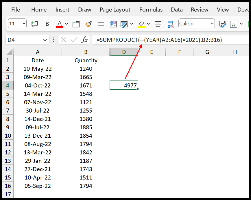
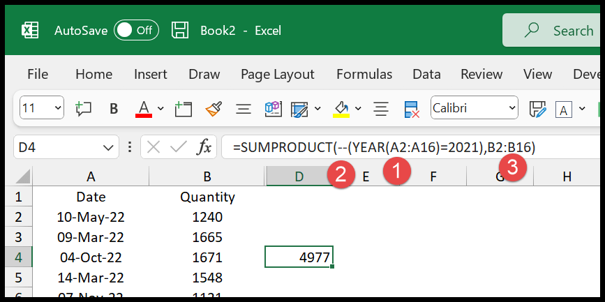
=SUMPRODUCT(--(YEAR(A2:A16)=2021),B2:B16)

To understand this formula, you need to use break it into three parts.

In the first part, you have the year function with a condition to check for the year 2021 in the date function. This condition returns an array of TRUE and FALSE according to the year that you have on the date. If a date has the year 2021, it returns TRUE, otherwise, FALSE.

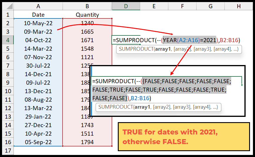
In the second part, you have two minus signs (–) which convert TRUE and FALSE values into 1 and 0, respectively.

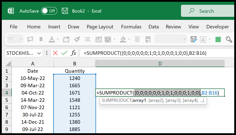
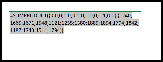
In the third part, you have the two arrays, one with the values 0 (for the year 2021) and 1 (for the years other than 2021), and the second array with the sum values from the range. SUMPRODUCT multiply both arrays with each other and they sum those values.

Now here’s one thing that you need to understand: When you multiply zero with any values, it returns 0. So, you are only left with the values where you have 1 in the first array.