Let’s say you organized a charity event and collected donations from different people. You have a list of those who provided their names and donations, while others chose to donate anonymously.
Your goal is to find out the total amount of donations from those who provided their names.
In Excel, you can use SUMIF to sum the value for the not blank cells; you need to specify a non-blank value (“<>” does not equal to – by using the greater than and lower than the operator) in the criteria argument of the function.
With this, SUMIF will look only for non-empty cells and only consider values from the [sum_range] according to that. Below, we have calculated the sum of donations with names.

Let’s write a formula for this…
Using SUMIF for Not Blank Cells
Here, we need to write a formula to add up the donations listed in column B, but only if the corresponding name in column A is not empty.
Quick Intro to SUMIF: The SUMIF function in Excel adds up the values in a range that meets a specified condition or criterion. It combines the functionality of the SUM and IF functions, allowing you to filter and sum data based on criteria.
- First, in the cell, enter the =SUMIF(.
- Now, in the criteria range, refer to the range A2:A13.
- Next, enter the criteria for not blank cells using “<>”.
- After that, in the [sum_range] argument, refer to the range B2:B13.
- In the end, enter the closing parentheses and hit enter to get the result.

When you enter the formula and hit enter, it returns the sum of the donation for only those cells where you have a name in the name column.
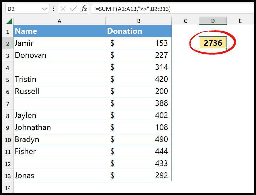
=SUMIF(A2:A13,"<>",B2:B13)
SUMIF function checks each cell in the range A2:A13 (criteria range). For every cell that is not empty (indicated by the “<>”), it includes the corresponding cell for donation amount from the same row in the range B2:B13.
It ensures that only the donations with a name are counted. In this case, the total is 2736, as shown in cell D2.
In the same way, if you want to sum non-blank cells using the SUMIFS instead of the SUMIF, you can write a formula like the following:
=SUMIFS(B2:B13, A2:A13, "<>")
Like SUMIF, this formula looks at each cell in A2 to A13. If a cell is not blank, it takes the values of the corresponding cells from B2 to B13 and adds them to the total. If a cell in A2 to A13 is blank, the corresponding cells in B2 to B13 are ignored.
=SUMIFS(B2:B13, A2:A13, "", C2:C13, ">10", C2:C13, "<=20")
When using the SUMIF, you can type the criteria directly into the formula or refer to a cell containing the criteria. Typing the criteria directly, like “<>,” is called using hard values.
This approach works perfectly but can make the formula less flexible. If you need to change the criteria, you must edit the formula every time, which can be time-consuming.
On the other hand, referring to a cell for the criteria makes your formula more dynamic. Instead of typing “<>” into the formula, you can type it into a cell and refer to that cell in the formula.
SUMPRODUCT to SUM Actual Non-Empty Cells
Let’s say you have a blank cell and a blank space in that cell. Now, this cell looks like an empty cell, but it is not empty.
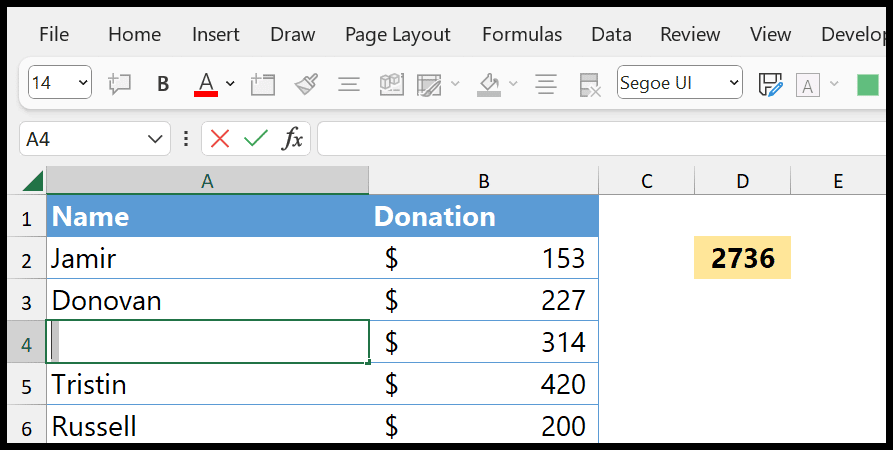
In this situation, SUMIF will also calculate that cell’s sum.
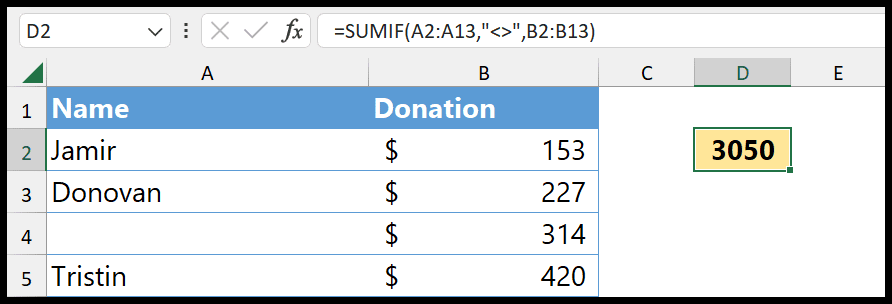
To deal with this problem, you can use a combination of SUMPRODUCT, LEN, and TRIM. With this combination, you can create an array formula. See the example below.
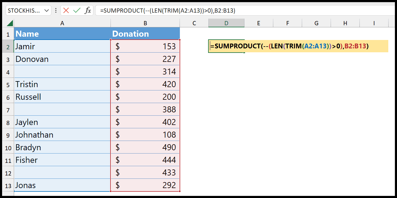
=SUMPRODUCT(--(LEN(TRIM(A2:A13))>0),B2:B13)
When you enter this function, it removes those blank spaces from the cells using TRIM. But there’s one thing that you need to know about SUMPRODUCT. It can take an entire array in a single cell without using the CTRL + ALT + ENTER keys.
Now, let’s break this formula into five small parts to understand it and see how this amazing formula works.
In the first part, we used the TRIM and referred to the entire name column. TRIM takes values from the column and removes space from the cells where you only have space(s). These are those cells that have no value but seem like non-blank cells.
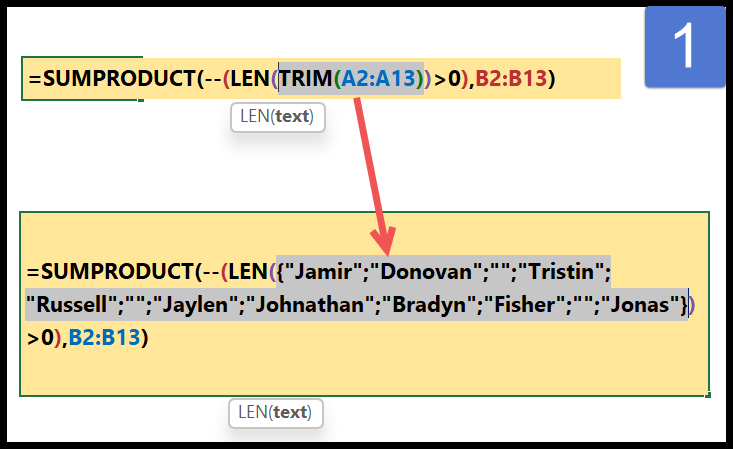
In the second part, we have LEN, which counts the length of the characters in the name column. For all cells where you don’t have any value, the count of the characters would be zero.

As you can see, we have values above zero for all the non-empty cells.
We used a greater than operator in the third part to compare the LEN and TRIM’s result returns. This operator converts the count into TRUE and FALSE. For a count above zero, it is TRUE, and otherwise, it is FALSE.

In the fourth part, we have a double minus sign that converts these TRUE and FALSE values into 0 and 1. For TRUE, a 0 and FALSE a 1.

After that, in the fifth part, we have SUMPRODUCT with two arrays. When these arrays are multiplied with each other, you get the sum only for the cells that are not blank and don’t have an invisible space.
Combining FILTER with SUM to Sum Not Blank Cells
Using the FILTER function with the SUM function can be a powerful way to sum up not blank cells in Excel. This method is beneficial in dynamic arrays where you want to sum only the cells that meet specific criteria, such as being non blank.
=SUM(FILTER(B2:B13, A2:A13 <> ""))
The FILTER function examines the range B2 to B13 and only includes values for which the corresponding cells in A2 to A13 are not empty.
It simply checks each cell in the range A2 to A13. If a cell is not blank, it takes the value from the same row in B2 to B13 and includes it in the sum. If a cell in A2 to A13 is blank, the value from B2 to B13 is ignored.