Use SUMIF to Sum Blank Values or Empty Cells

Let’s say you are coordinating a fundraising campaign for a non-profit organization. You have an Excel worksheet where column A lists donor names, column B shows the donation amounts, and some names in column A are left blank – perhaps because some donors chose to remain anonymous or their details were not captured during the donation process.

So here we need to sum values for the cells which are blank to sum the amount from the anonymous donors.

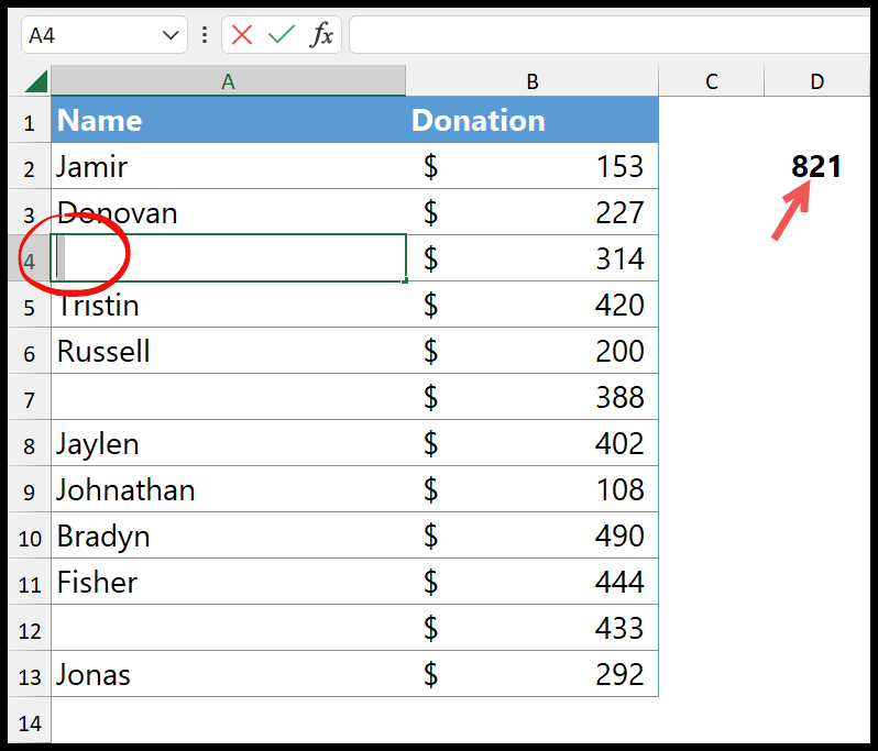
Now, to use SUMIF to sum values for the blank criteria, you just need to specify a blank value in the criteria argument in the SUMIF function. With this, tell Excel to only consider cells where there’s no value. In the example, below we have three blank cells in the name column for which we need to sum the donation amount.

In this tutorial, we will learn to use SUMIF or SUMIFS function to sum for blank values.

Write a formula to use SUMIF for Blank Values

As I have mentioned, for this, you can use the SUMIF function to sum the values in column B.

1. First, enter SUMIF in a cell where you want to calculate the sum.
2. Now, refer to the Name column where you have blank cells.
3. After that, enter double quotation marks (starting and closing).
4. Next, refer to the Donation column from where you need to sum the values.
5. In the end, hit enter to get the result.

=SUMIF(A2:A13,"",B2:B13)

• Name Range (A2:A13): This is the list of donor names. The formula looks here to find blank spaces where names should be.
• Criteria (“”): The criteria is set to find the blank cells. When it finds a cell without a name, it means the donation was made anonymously.
• Sum Range (B2:B13): The donation amounts are listed here. The formula adds up the donations that match the blank name criteria from the range above.

Create a Dynamic Formula for SUMIF Blank

To make a formula dynamic, enabling it to automatically adjust as data is added or removed from your dataset, you can use OFFSET function along with COUNTA or INDEX in SUMIF.

=SUMIF(OFFSET(A1, 1, 0, COUNTA(A:A) - 1, 1), "", OFFSET(B1, 1, 0, COUNTA(B:B) - 1, 1))

This formula uses COUNTA(A:A) – 1 to count all the non-empty cells in column A, subtracting one to exclude a header if it’s present. This gives us the number of actual data entries. Then, OFFSET(A1, 1, 0, …) is used to start the range from the second cell (A2) and extend it to cover the number of entries we counted.

The same approach is applied to column B, ensuring the sum range aligns with the actual data entries in column A. This way, the formula dynamically adjusts to include just the right amount of data as it changes, like when new values are added or existing ones are deleted.

A Problem You Might Face

There might be a situation where you have a range of cells where you have a cell or multiple cells with space as a value in the cell which looks like a blank cell, but not a blank cell. In that case, SUMIF will ignore that cell and won’t include it while calculating the sum.

Here, you can create a formula with the help of SUMIFS and SUM to create a SUMIF OR.

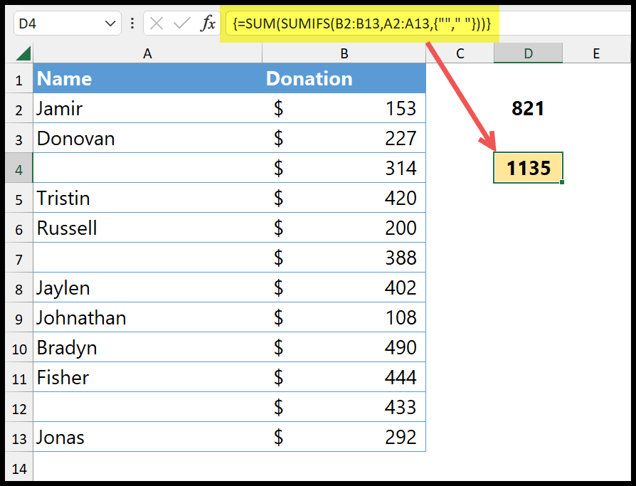
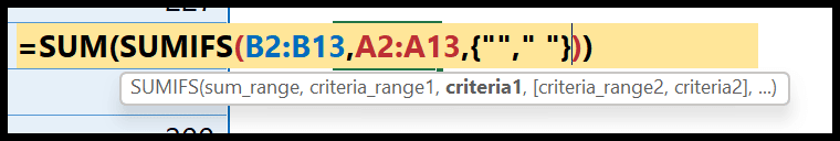
In this formula, you need to specify two criteria in the criteria1 argument using curly brackets.

• Space
• Blank

When you do this, SUMIF considers both criteria simultaneously. And to get the result, you need to enter it as an array formula (use Ctrl + Alt + Enter you can learn more about it here.) .

=SUM(SUMIFS(B2:B13,A2:A13,{“”,” “}))

And you can also use SUMPRODUCT for this:

=SUMPRODUCT(--(LEN(TRIM(A2:B13))=0),B2:B13)

• TRIM(A2:B13): This function is a practical tool that removes any leading or trailing spaces within cells in the range A2 to B13. As we work with donor names and donation amounts, it’s more appropriate to apply this function to just the donor names (e.g., TRIM(A2:A13)).
• LEN(TRIM(A2:A13))=0: This part of the formula is straightforward; it simply calculates the length of the trimmed content of each cell in the specified range. If a donor’s name cell is blank, even after trimming, its length will be 0.
• –(LEN(TRIM(A2:A13))=0): The double negation (–) converts the Boolean values TRUE and FALSE into 1s and 0s, respectively. This results in an array where each element is 1 if the corresponding donor name is blank (after trimming) and 0 otherwise.
• B2:B13: This range contains the donation amounts corresponding to each donor name listed in A2 to A13.
• SUMPRODUCT(–(LEN(TRIM(A2:A13))=0),B2:B13): SUMPRODUCT multiplies arrays together and then sums the result. This formula multiplies the array of 1s and 0s generated from donor name conditions by the corresponding donation amounts. Only the donations where the donor name is blank are summed because multiplying by 0 nullifies the other values.

Other Example of using SUMIF for Blank

Combine SUMIF with ISBLANK Inside an Array Formula

This is an array formula that sums values in B1:B13 where A1:A13 cells are blank.

=SUM((ISBLANK(A1:A10) * B1:B10))

Sum Blank values while considering one more Condition

=SUMIF(B2:B13, "", IF(ISBLANK(A2:A13), 50, A2:A13))

Sum alternate values for blanks

=SUMIF(B2:B13, "", IF(ISBLANK(A2:A13), 50, A2:A13))

Sum a constant number for each blank cell in a range

=SUMIF(A1:A13, "", 1)

Sum with indirect reference to blanks in adjacent cells

=SUMIF(B1:B10, "", OFFSET(A1:A10, 0, 1))