

You can nest VLOOKUP inside SUMIF’s criteria argument when the value you need to sum by isn’t the one you have. The formula is =SUMIF(A2:A13,VLOOKUP(B15,D2:E7,2,0),B2:B13): VLOOKUP takes the product name in B15, returns its product ID from the reference table, and SUMIF then totals the quantity column for every row carrying that ID.
So a user picks a readable name — ideally from a dropdown in B15 — while the data itself stores codes. The same works across sheets by adding the sheet name to the lookup range: =SUMIF(A2:A13,VLOOKUP(B15,Sheet2!A2:B7,2,0),B2:B13).
Two things to guard against. If VLOOKUP can’t find the name it returns #N/A, and SUMIF passes that straight through instead of returning 0 — wrap it as =IFNA(SUMIF(...),0).
And the ID VLOOKUP returns must match the ID column exactly: a trailing space or a code stored as text on one side gives you 0 with no error.
Yes, you can combine VLOOKUP and SUMIF. In SUMIF, there is a criteria argument in which you can use VLOOKUP to create a dynamic value. This will allow you to change the criteria by changing the lookup value in the VLOOKUP. The use of this combo formula is unique.
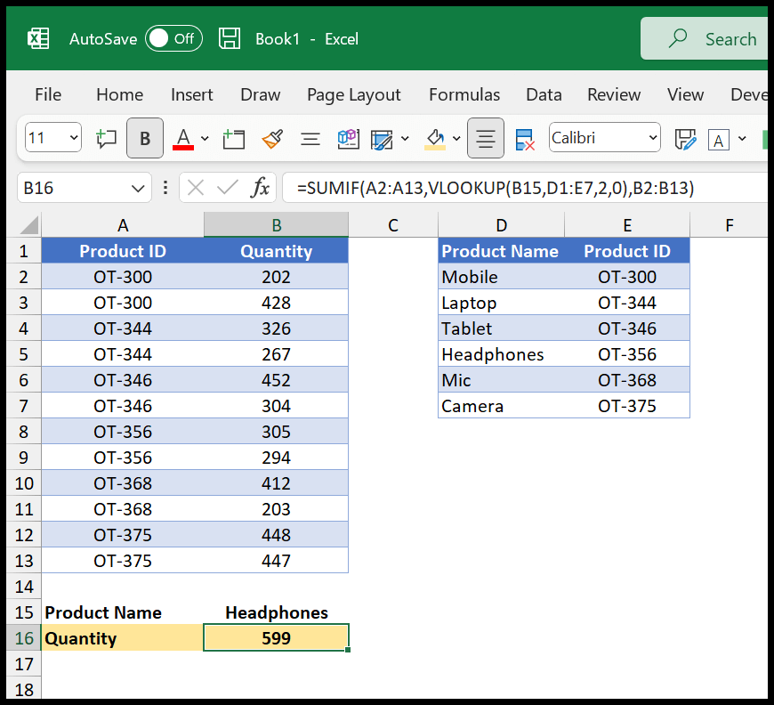
In this tutorial, we will learn to combine SUMIF and VLOOKUP to create a formula.
Combine SUMIF and VLOOKUP
- First, in a cell enter “=SUMIF(“, for the range argument, refer to the product ID range that you have in table1.
- After that, in the second augment, you need to use the VLOOKUP function to lookup for the product ID by using the product name from the cell above.
- Next, in the third argument of the SUMIF, refer to the quantity column to use as a sum_range.
- In the end, enter the closing parentheses and hit enter to get the result.
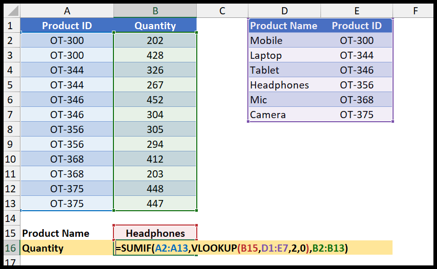
=SUMIF(A2:A13,VLOOKUP(B15,D1:E7,2,0),B2:B13)

How this Formula Works
Let’s break this formula into three parts: In the first part, you have specified the range where you have the product ID.
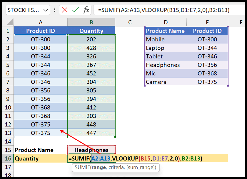
In the second part, you have the VLOOKUP that takes the product name from cell B15 and lookup it in the table2. For Headphones, we have the Product ID OT-356.
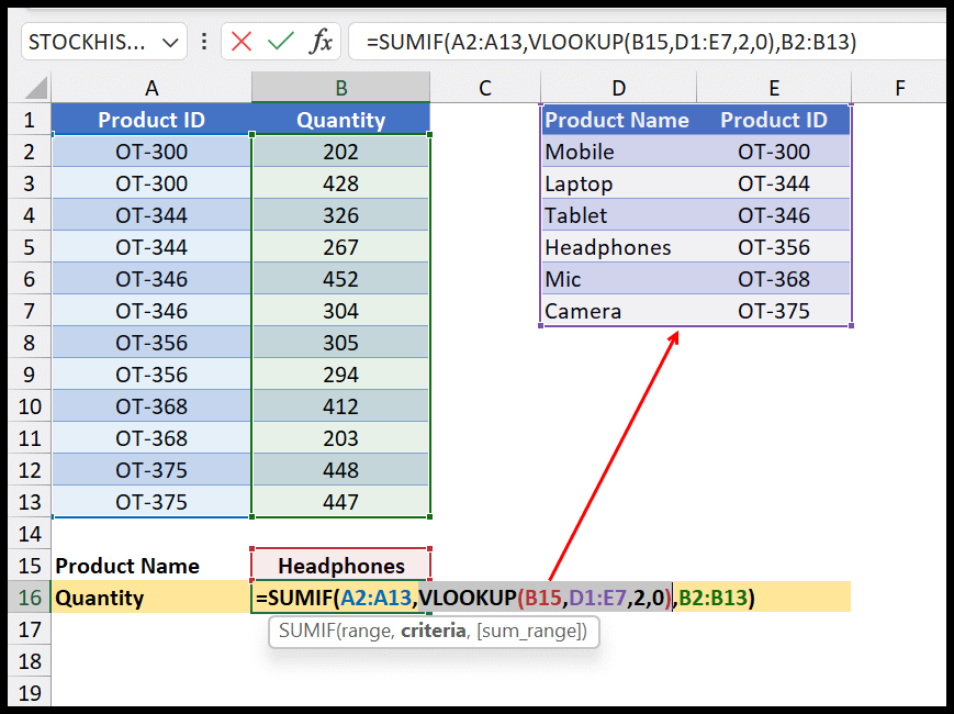
In the third part, we have the quantity column as sum_range.
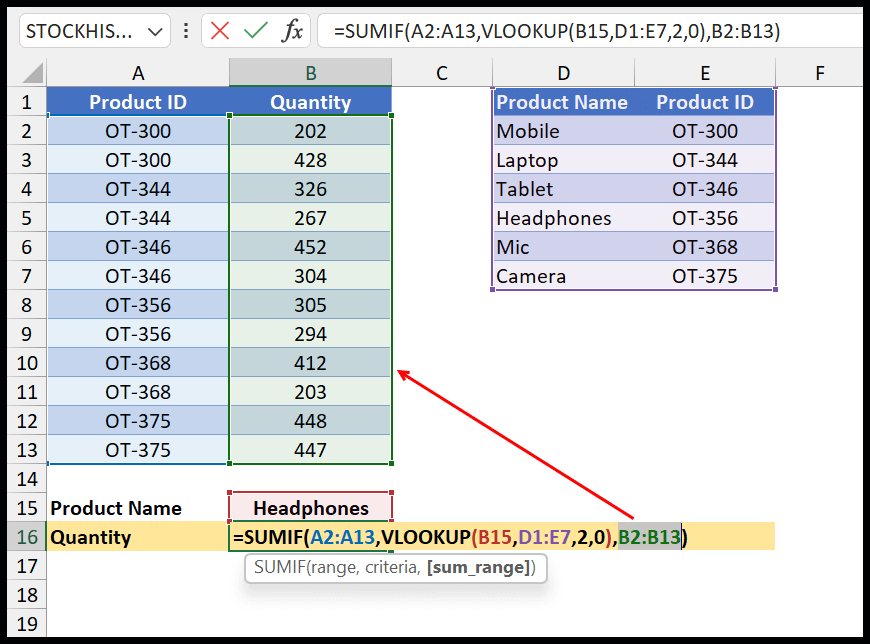
In short, VLOOKUP helps you find the Product ID with the Product Name and then SUMIF takes that Product ID and looks it up in the Product ID column, and then sums values from the Quantity column.
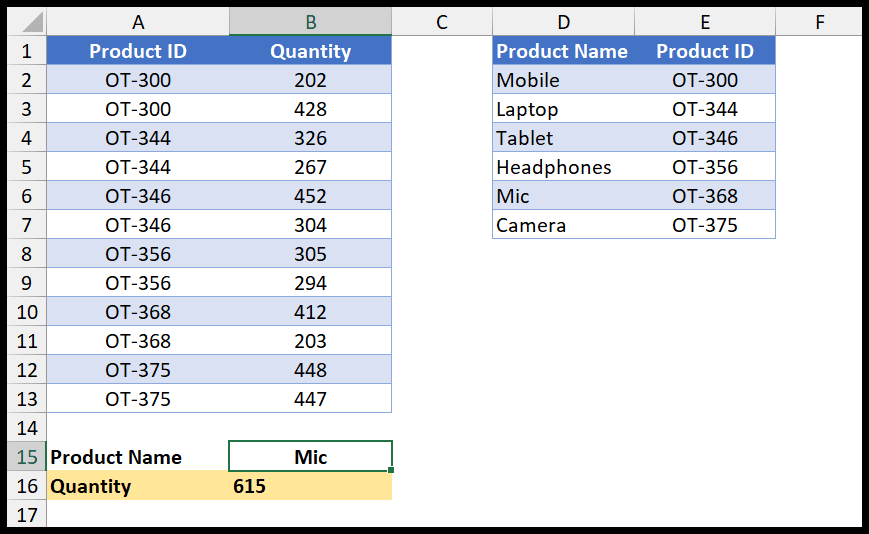
As I said, when you use SUMIF and VLOOKUP, this makes your formula a dynamic formula. When you change the product name in the cells it changes the result.
SUMIF and VLOOKUP in Multiple Sheets
You can use this combination even when you have both tables in multiple sheets differently.
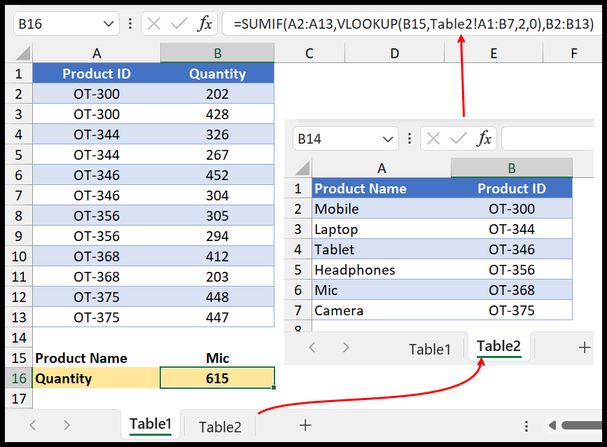
In the above example, you have the product name table on a different sheet.
Get the Excel File
Related Formulas
- Sum Greater than Values using SUMIF
- Sum Not Equal Values (SUMIFS) in Excel
- SUMIF / SUMIFS with an OR Logic in Excel
- SUMIF with Wildcard Characters in Excel
- SUMIFS Date Range (Sum Values Between Two Dates Array)
- Sum IF Cell Contains a Specific Text (SUMIF Partial Text)
- Sum Values Based on Year (SUMIF Year)
- SUMIF By Date (Sum Values Based on a Date)
-
Back to the List of Excel Formulas
Written by
Puneet Gogia
Microsoft MVP — Excel · Founder, Excel Champs
Twelve years of teaching Excel, and a decade before that using it as a data analyst. Every tutorial here is written from a file I actually built.