How to Refresh a Pivot Table in Excel

1. Use the "Refresh All" button (all pivots, one click)

The Refresh All button is the simplest way to update every pivot table in a workbook at once.

• Select a pivot table. Click any cell inside one of your pivots — this tells Excel your next action is about pivot tables.
• Go to the PivotTable Analyze tab. This tab only appears on the ribbon when a pivot is selected.
• Open the Refresh drop-down. In the Data group, click the small arrow on the Refresh button.
• Choose "Refresh All". This updates every pivot table in the workbook, not just the selected one.

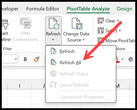
You can also skip the pivot entirely and use Data tab ➜ Refresh All (in Queries & Connections). Prefer the keyboard? Press Alt A R A in sequence to fire Refresh All without touching the mouse.

2. Refresh all pivots automatically when you open the file

If you'd rather not remember to refresh at all, set the workbook to refresh its pivots every time it opens. It's a one-time setup.

• Select any pivot table (a single cell inside it is enough).
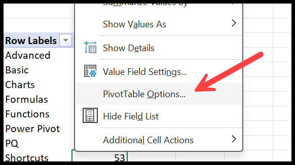
• Right-click and choose "PivotTable Options…".
• In the dialog box, go to the Data tab and tick "Refresh data when opening the file". Click OK.

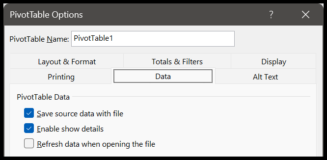
One caveat: on large workbooks this refresh runs before the file is usable, so it can noticeably slow down opening. For heavy models, I'd keep this off and use a manual Refresh All (or a button) instead.

3. Refresh all pivots with a keyboard shortcut

Once the workbook is open, refresh every pivot table by pressing:

Ctrl + Alt + F5

This runs the same Refresh All as the ribbon. Depending on the size of your pivots and your machine, it may take a moment.

On a Mac: there's no single shortcut to refresh all pivots. Cmd + Shift + F5 refreshes the selected pivot — for all of them, use Data ➜ Refresh All from the ribbon.

3. Refresh all pivots with a keyboard shortcut

Once the workbook is open, refresh every pivot table by pressing:

Ctrl + Alt + F5

This runs the same Refresh All as the ribbon. Depending on the size of your pivots and your machine, it may take a moment.

On a Mac: there's no single shortcut to refresh all pivots. Cmd + Shift + F5 refreshes the selected pivot — for all of them, use Data ➜ Refresh All from the ribbon.

4. Refresh all pivots with VBA

If you want a one-click macro (or you're already automating the workbook), VBA is the cleanest route. To refresh every pivot, query and connection in the workbook, this single line does the job:

Sub RefreshAllPivots()
    ThisWorkbook.RefreshAll
End Sub

ThisWorkbook.RefreshAll is the same as clicking Refresh All on the Data tab — it walks the whole workbook, so you don't have to name a single sheet or pivot.

If you want to refresh pivots only (and leave other data connections alone), loop the pivot caches instead — pivots that share a cache refresh together:

Sub RefreshAllPivotCaches()
    Dim pc As PivotCache
    For Each pc In ThisWorkbook.PivotCaches
        pc.Refresh
    Next pc
End Sub

And if you only need the pivots on the sheet you're looking at, keep it local:

Sub RefreshPivotsOnThisSheet()
    Dim pt As PivotTable
    For Each pt In ActiveSheet.PivotTables
        pt.RefreshTable
    Next pt
End Sub

Refresh only specific pivot tables with VBA

To update just a few named pivots, list them explicitly:

Sub RefreshSelectedPivots()
    With ActiveSheet
        .PivotTables("PivotTable1").RefreshTable
        .PivotTables("PivotTable2").RefreshTable
        .PivotTables("PivotTable3").RefreshTable
    End With
End Sub

Change the names to match your workbook (you'll find them on the PivotTable Analyze tab, in the PivotTable Name box).

To run any of these automatically on open, put the code in the ThisWorkbook module inside a Workbook_Open event:

Private Sub Workbook_Open()
    ThisWorkbook.RefreshAll
End Sub

Note: older tutorials use a macro named auto_open for this. Workbook_Open is the modern equivalent and is what I'd use today — auto_open only survives for backward compatibility.

Bonus: refresh pivots automatically whenever the data changes

Opening the file isn't the only trigger. If you want your pivots to never sit out of step with the source, refresh them whenever the sheet changes. Put this in the code module of the sheet that holds your source data:

Private Sub Worksheet_Change(ByVal Target As Range)
    Application.EnableEvents = False
    ThisWorkbook.RefreshAll
    Application.EnableEvents = True
End Sub

The EnableEvents = False / True lines matter: without them, the refresh can re-trigger the change event and send Excel into a loop. A few readers in the comments swear by this — it means you're always looking at current numbers.

Which method should you use?

Understanding the source data (and why refresh sometimes "doesn't work")

The source data is the original range, named range, or Excel Table your pivot is built on — every row and column it summarises.

Here's the gotcha that trips most people up: Refresh only re-reads the range the pivot already knows about. If you add new rows or columns below or beside that range, refresh won't pick them up, and it looks like the button is broken.

The fix is to base your pivot on an Excel Table (select your data and press Ctrl + T) before you create the pivot. A Table grows automatically as you add data, so a plain refresh always captures the new rows. If your pivot is on a fixed range, you'll instead need to update the source via PivotTable Analyze ➜ Change Data Source.