How to Filter a Pivot Table in Excel (Filter Pivots)

In a pivot table, filters allow you to manage and visualize your data more effectively. You can narrow down the data that is displayed based on specific criteria.

Type of Filter in a Pivot Table

In a pivot table, there are several types of filters you can use to filter data:

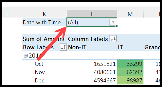
1. Report Filter

The Report Filter is like a main filter in a pivot table. it is at the top of the pivot table. It’s an especially useful feature when you need to create distinct reports. For instance, if you have a pivot table that includes sales data from various states, you can use the Report Filter to create separate reports for each state.

2. Label Filter (Columns & Row)

This type of filter allows you to filter data based on the labels in the pivot table. You can use a variety of conditions, such as ‘equals’, ‘does not equal’, ‘begins with’, etc. It’s particularly useful when you have text-based data and want to narrow a pivot’s view to specific categories or items.

3. Manual Filter

This filter allows you to manually select or deselect items in the pivot table for display. It lets you hand-pick the data points you wish to see and hide the rest. This can be useful when focusing on specific data points.

4. Search Filter:

This filter allows you to search for specific items in the pivot table. It’s a powerful tool when you’re dealing with large data sets and need to locate specific data points quickly.

5. Value Filter

This filter allows you to filter data based on the numerical values in the pivot table. You can use conditions like ‘equals’, ‘does not equal’, ‘greater than’, etc. This is particularly helpful when analyzing data that meets certain numerical conditions.

6. Date Filter

This filter allows you to filter data based on dates. It provides options to filter by year, quarter, month, and day. This is particularly useful when dealing with date/time-based data; you only wish to see data from a particular period.

7. Top 10 Filter

This filter allows you to display the top or bottom ‘n’ items based on the value field. This is a quick way to identify the highest or lowest data points in your pivot table, which can be very helpful for identifying trends or outliers.

Using Report Filter in a Pivot Table

Report filters are amazing when you must filter data based on two or more criteria. To add a column to report filters.

• First, click anywhere on the pivot table and activate the field list option.
• Now, select the column which you want to add to report filters. Here we will add industry.
• Here drag/add the column Industry to filters in pivot table fields.
  
• Now the pivot table will look like this.
  
• After this click on the little drop-down next to industry.
  
• Here you will get a list of the industries in your data.
• Now, to select multiple, tick mark on the bottom “Select multiple”.
  
• In the end, if you have a long list, you can simply type in the search box. Here we are typing “Med”, and all the industries with “Med” text are filtered.
  
• Here, you can deselect or select the industries you want to filter.

Search Box to Filter Data in a Pivot Table

The search box is the easiest and most handy filter.

• First, click inside the search box.
  
• Here start typing text to filter the data.
  
• After this, you will see that the data is filtered by the text “ENT”. Here you will notice that all the items which have “ENT” are listed below.
• Untick the items you do not need.
  
• Hit OK.

Clear Filter from a Row or a Column in a Pivot Table

• Another way of doing this is simply to click on the arrow next to the column “Name”.
  
• Now click on the “Clear Filters from “Name””.
  

Other Method

• Click on the row/column where you have applied the filter and right-click.
  
• Here look for the option of “Filter” and click to get the option of “Clear Filter from Name”.
  

Clear All Filters

If you want to clear all the filters irrespective of columns and rows, follow the steps below.

• To start with, click on the pivot table to activate analyze tab.
  
• Now, click on the little down arrow next to clear.
  
• At last, click on “Clear Filters”. This will clear all the filters applied to the pivot table (in other words, it will reset the filters).