Pivot Table Formatting

Working on a pivot table is quite interesting but sometimes it feels boring using the same inbuilt colors and layouts. If you are very particular about the aesthetics and color layouts in your report, here you need to know a few things about a pivot table.

Default Style Options

There are a few options available on the ribbon once you have pivot table on your worksheet.

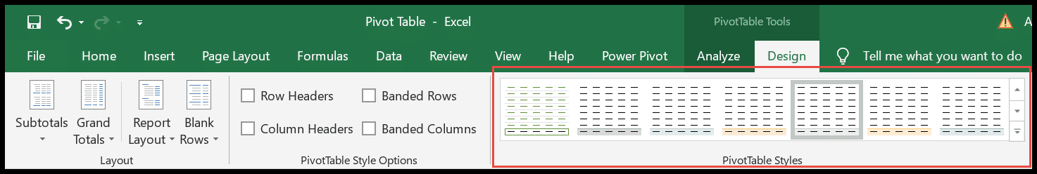
You can choose between many colors and themes (light, medium and dark) from the little drop-down arrow.

Quick Tip: The layout options change as you change the PivotTable Style options and the layout.

Change Pivot Table Formatting

Now to choose a particular style as a default for your PivotTables use the following steps.

1. First, click anywhere on the PivotTable to activate the Design tab in the ribbon.
   
2. Now, in the PivotTable Style gallery, right-click on the style that you want to set as the default.
   
3. In the menu, click “Set As Default
   ”.
4. This will make the selected style a default style.

Duplicate and Modify

Let’s begin with creating it from scratch.

1. Click anywhere on the PivotTable to activate the design tab.
2. Now, click on the small drop-down arrow in the designs to scroll to the end.
   
3. Here click on the “New PivotTable Style”.
   
4. Now, a pop-up window will open “New PivotTable Style”.
5. Rename the PivotTable in the “Name Field”
6. Select an element to format and click on the “Format” button.
7. In the end Click OK to create your style.
8. In case you want to keep the style for future pivots, just tick mark the option in the end as mentioned in the screenshot.
   

Now let’s edit a given default style. This is almost the same as creating a new style.

1. To start with, right-click on the style that matches your requirement.
   
2. Now click on the duplicate to open a dialogue box “Modify PivotTable Styles”.
   
3. Now, you guys know what to do.

Copy the Layout to a Different Worksheet

Since we have invested a lot of time in creating our custom layout, let’s copy it to another worksheet to save energy.

1. To start with, open the workbook with a custom layout.
2. Next, open a new workbook where you want to copy the custom layout.        
3. Now place both the workbooks adjacent so that both are visible on the screen (Tip: Use Arrange all options given in View in the ribbon).
   
4. Use “Arrange All” options given in View in the ribbon.
   
5. In the end, press ctrl and drag the layout sheet to the new workbook.
6. Boom!! The custom layout is copied to the new workbook.
7. Now you can delete the sheet you dragged to the workbook.

More on Pivot Table

Sort a Pivot Table | Refresh a Pivot Table | Pivot Table Keyboard Shortcuts  |Move a Pivot Table | Filter a Pivot Table | Count Unique Values in a Pivot Table | Change Pivot Table Data Source| Add or Remove Grand Total in a Pivot Table | Add Ranks in Pivot Table | Insert Calculation in Pivot Table | Refresh All Pivot Tables  | Automatically Update a Pivot Table | Running Total in a Pivot Table | Conditional Formatting to a Pivot Table | Pivot Table from Multiple Worksheets | Group Dates in a Pivot Table | Connect a Slicer with Multiple Pivot Tables | Pivot Table Timeline