SUMPRODUCT is one of the most important Excel functions. The best part about it is, that you can modify it in several ways.
And one of its powers which I have discovered recently is: Using it as SUMPRODUCT IF In short, a Conditional SUMPRODUCT.
Well, as you know, you can use SUMPRODUCT to multiply and sum specified ranges or arrays. With a conditional SUMPRODUCT, you can multiply and sum those ranges which meet the criteria.
Yes, you heard it right. And you know the best part? There is no need to use the IF function for this. Isn’t it awesome?
Yes?
So today in this post, I’d like to share with you a problem and a simple way to use SUMPRODUCTIF to solve it.
So be with me to learn one of the most amazing Excel formulas and make sure to download sample files.
How I Got to Know About this Conditional SUMPRODUCT
First thing first.
Yesterday, I got a mail from one of my subscribers. She wanted to create a conditional statement with SUMPRODUCT and IF to get data from a table.
Here is the mail which I have received:
Hey Puneet, I need your help. Is there any way to combine SUMPRODUCT IF? I have some data in a table, and I want to get the product of two columns meeting criteria. Please help me out.
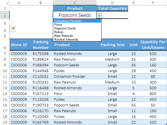
Along with the mail, I got an Excel file from her with the following components. You can download this file from here to follow along.

- Stock Data: This table is stock data that is stored in different stores of her company. It has the product name, units in stock, and weight per unit.
- Drop-Down List: A drop-down menu to select a product.
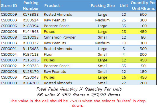
From this table, she wanted to get the total quantity of a product (units * weight per unit) by selecting the dropdown. For example, if she selects “Pulses”, the total quantity in the cell should be total by multiplying units by the quantity per unit.
Please note down, that a product name is a condition here.

Solution with SUMPRODUCT IF
At that time, I was sure about one thing to get the sum of the product of arrays or ranges we can use SUMPRODUCT.
But here, the game was to get the sum by multiplying the total of units and quantity per unit only for the cells that meet the criteria.
And the formula we can use:
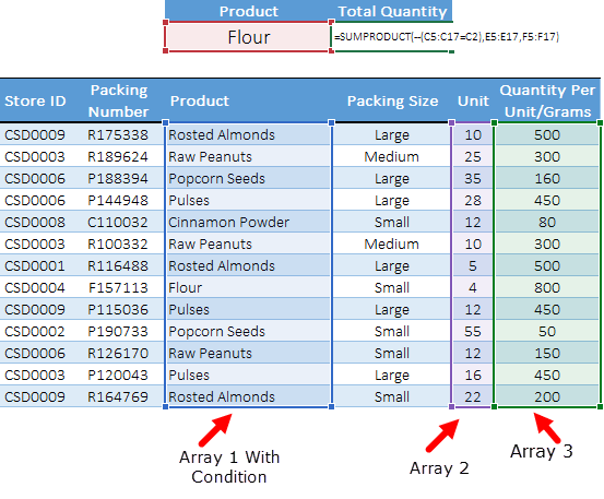
=SUMPRODUCT(--(C7:C19=C2),E7:E19,F7:F19)
Now, when you select an entry from the drop-down list, this formula will only return the product for cells that meet the criteria.
Hey, wait for a minute: Just like this formula, I have listed a few more smart formulas which can amaze you.
- Conditional Ranking in Excel using SUMPRODUCT Function
- How to use MAX IF Formula in Excel
- How to use OR Logic in COUNTIF/COUNIFS in Excel
- How to use SUMIF / SUMIFS with an OR Logic in Excel
How it Works
As you already know, SUMPRODUCT can work with arrays. So in the above method, we have used three arrays to get the product of values.

The formula works in the following way.
1. Creating a Condition
First, we have an array to check the condition of the product name. It will check the values from the product column, and return TRUE for the matched values, and FALSE for others.

2. Using Double Minus Sign
Now, the next thing is to convert TRUE-FALSE values into 0-1 so that we can use them in the calculation. And for this, we have used the double minus sign before the first array.

3. Multiplying Arrays
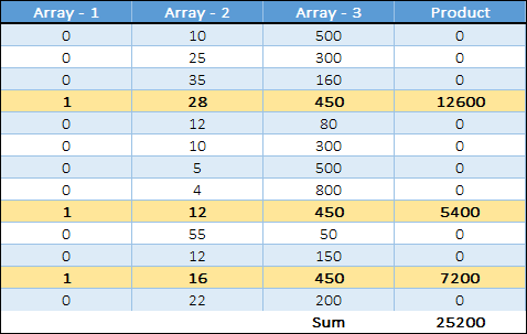
After converting TRUE-FALSE into 0-1 the array will look something like this. Here all the values where criteria are not met, we have zeros.

Remember, when anything multiplies with zero it returns to zero. In this way, we get the product for only those cells where we have 1. In short, where the condition is met.
Get the Excel File
Conclusion
The best part about using this conditional SUMPRODUCT is you don’t need to use IF and all the calculation is in a single cell. As I said SUMPRODUCT is one of the most powerful functions and this is the best thing you can do with its powers.
Now tell me one thing.
Have you ever tried using a condition in SUMPRODUCT before?
Please share your views with me in the comment section. I’d love to hear from you and please don’t forget to share it with your friends, I am sure they will appreciate it.
This post was incredibly helpful! I had been struggling to create conditional formulas in Excel, and using SUMPRODUCT IF really simplifies the process. The step-by-step examples made it easy to follow. Thanks for sharing!
I found your explanation helpful.
I have been using a similar formula and it worked a few months ago, but now it doesn’t work.
The older spreadsheets still work as they did before as long as I don’t bring in new data
The new files don’t.
I think something has changed within excel.
If you think you can help, let me know how to send you the files.
Fingers crossed
Hi Puneet,
This formula awesome!.
What if there is 1 more criteria need to be match(e.g. Cost Center with same products).
Much appreciate if you can advise this.
hi
can any one help to get the available qty of a part
table is like below
a1,a2,a3,a4 | available Qty1| available Qty2 | etc
Inv
A1 | 24
A2 | 30
A3 | 24
A4 | 15
Price so on so
Hi Puneet,
I want help with using sumproduct formula.
for eg
Item 100 piper has two serving (pegs) sizes (30 ml and 60 ml).
On a day sale is
30 Ml = 4 pegs = 120 ML
60 ml = 2 pegs = 120 ML
Total = 240 ML
What I want is how to apply the formula sumproduct so that
the sum comes in one place
Mohit, this is how I have used the example in my explanation. try to use the sample file that I have shared. let me know if you need further help. 🙂
I’m looking to use sumproduct to return a cumulative total or a zero for monthly totals year-to-date, January thru December, for months less than or equal to the current month or for months with no values which would be future months. I’m not seeing and examples in my search, see below:
Jan Feb Mar Apr May Jun Jul Aug Sep Oct Nov Dec
5 5 5 5 5 5 5 0 0 0 0 0
Desired results:
Jan Feb Mar Apr May Jun Jul Aug Sep Oct Nov Dec
5 10 15 20 25 30 35 0 0 0 0 0
All attempts using conditional operators — , etc have returne #Value! or other error while using the * returns:
Jan Feb Mar Apr May Jun Jul Aug Sep Oct Nov Dec
5 10 15 20 25 30 35 35 35 35 35 35
Do not want the existing cumulative total to be repeated in future months that have no zeros i.e. no monthly totals yet.
I would solve this different:
my excel is in german so i am not really sure about the right comands but i will try.
if(month(today())>Month(1 & A1); 5*Month(1 & A1); 0)
A1.value = Jan in your example
In the same example if I have multiple stores how to get total weight of the store which I will select from drop down.
it should be based on below conditions
Store
Name of the product
Product quantity
Product weight
Store Total Quantity
Abc 0
Store Packing Number Product Packing Size Unit Quantity Per Unit/Grams
abc R175338 Rosted Almonds Large 10 500
xyz R189624 Raw Peanuts Medium 25 300
rmp P188394 Popcorn Seeds Large 35 160
abc P144948 Pulses Large 28 450
xyz C110032 Cinnamon Powder Small 12 80
please help and reslove
Hey,
Thanks for this great explanation on this function. This is what I will probably need but I see SUMPRODUCT thinks with ‘and’ by default. Unfortunately, I need the ‘or’ version if feasible. The task is simple, I have a row of values (1,2,3,4,5) and a sheet full of values on the other side. I want to tell Sumproduct to count the number of rows in the table where any of my numbers occur. Each row should only be counted once regardless of how many matches found there. For this I will need to tell excel to “count rows in the range where any of the values from the 1-2-3-4-5 occur.” Would this be possible? I have searched so many forums and explanations on this function, no solution found. Each of them counts the number of cells (not the rows) or counts them only if multiple criteria are met at the same time. None of these fit my purpose. Thanks.
I have discovered this amazing function, but my Mac struggles with it. I would like to multiply array 1 by array 2. One of these is a lookup in a table based on array 2.
Is this possible?
The other problem is with gaps or blanks in arrays, do these disable the SUMPRODUCT function.
would this work on product() too? I am trying to calculate compounded returns and need to conditionally select daily data for each month and compound it to a single value.
share a snapshot of data.
Dear Sir,
Please provide me advance nested Index and matching formula. i have lot of doubt while using this.
Regards
Maheswar
Hi, Puneet, May I ask you how to filter a pivot table with “*”
say, I wish to filter a field with items start with “CS”
Thanks!
Puneet …. You are the best. …. A gem !!!
Thanks for your words.
What if i want to use the sumproduct formula to count zeros?? i’m making a form that needs to count days worked and days not worked, i have multiple criteria and it worked perfectly to sum the days worked…