
In this tutorial, we will learn to calculate the average of the time values you have in a range of cells.
Formula to Average Time
In the following example, you have three-time values in column A in the range A1:A3. Now, you need to calculate the average of these time values.

For this, you need to use the AVERAGE function.
- Enter the average function in a cell by using the equal sign.
- Then enter the AVERAGE function and start parentheses.
- Refer to the range where you have the time.
- In the end, enter the closing parentheses and hit enter to get the result.
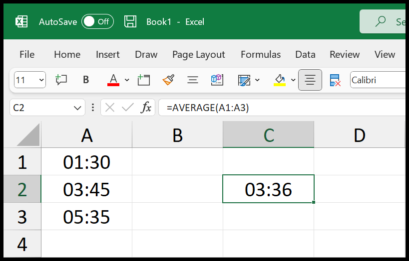
=AVERAGE(A1:A3)In the cell where you want to calculate the average of the time, you need to make sure to have the time format on that cell. Even if you don’t change the format, Excel is smart enough to change this format for you when you enter the formula in it.
Understand Time in Excel
In Excel, when you enter time in a cell, Excel formats it automatically. There are two ways to format a time value: a 12-hour format and a 24-hour format. When you are averaging time and have a 12-hour format, you need to be a little cautious.
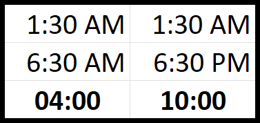
Above we have two different times one is 6:30 AM and the second is 6:30 PM. That’s why the average is different with both formulas.
Why I’m Getting #DIV/0! Error While Averaging Time
If your time values are stored as a text value in the cell, you might face #DIV/0! error. Below we have a list of time values that are saved as text and on averaging we are getting an error.

To solve this problem, you can use the following formula.
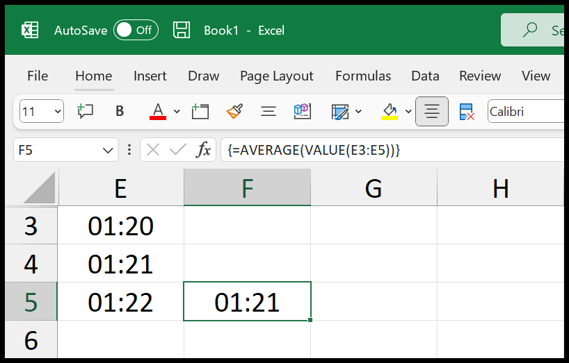
You need to enter this formula as an array formula by using Ctrl + Shift + Enter.