Calculate the Cumulative Sum of Values in Excel (Running Total)

The best way to calculate the Cumulative Sum of Values or a running total is to use the SUM function.

You need to refer to the previous and current values in the formula and then drag that formula to all the cells up to which you want to calculate the running total (cumulative sum).

This tutorial will teach us to write this and a few other formulas to deal with different situations.

Formula to Calculate a Cumulative SUM (Running Total)

You can use the following steps:

1. First, enter the sum function in cell C2.
2. After that, refer to the range B2:B3. This range includes the quantity for day 1 and day 2.
3. Now, use the dollar sign before the row number of the cell reference.
4. Next, enter the function to get the cumulative total for two days (1 and 2).
5. In the end, drag the formula to the column’s last cell to get the running total for all the days.

When you use the dollar sign, the first cell freezes, and each cell’s cumulative sum for all the previous days is calculated.

Cumulative Sum by Date (Date Running Total)

Now, let’s say you have the data with dates and quantity. See the example below; we have two columns of data.

However, these dates are not in the sequence. So, the first step is to sort the data into a series of dates.

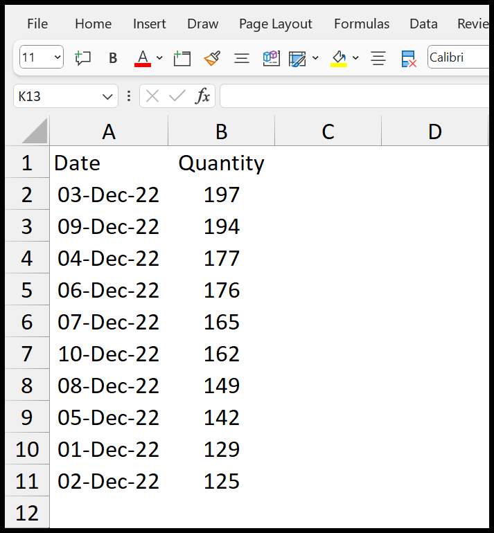
First, you need to sort data from old to new to get the date-wise running total.

To open the sort dialog box, use the keyboard shortcut (Alt + S + S) or go to the Data Tab > Sort Button.

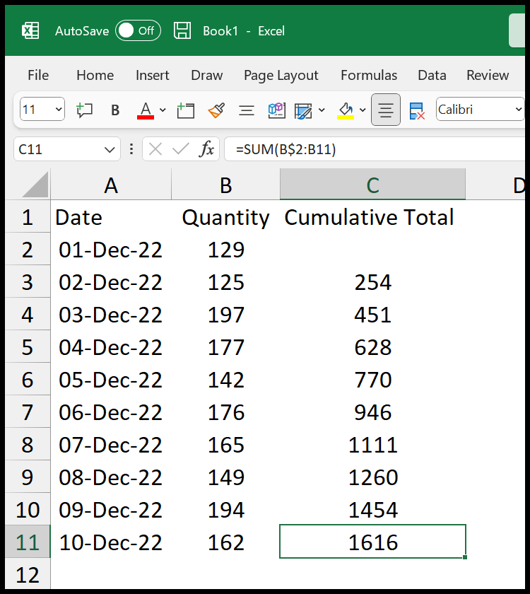
After that, you can enter the sum formula in the C3 cell. For this, you need to refer to the range B2:B3.

But in the first cell of the range address, you need to use the dollar sign to freeze the cell.

Ultimately, once you enter the formula, drag it up to the last cell with the date to get a running total for all the dates. The example below shows the running total from cell C3 to C11.

Cumulative Sum by Month

In the following example, we have dates in column A.

But we want to calculate the running total based on the months instead of the dates.

You must first add a separate column with month names to do this.

In the next column, enter the following formula, referring to the date and quantity columns from the original table.

=SUMPRODUCT(--(TEXT($A$2:$A$11,"MMM")=D2),$B$2:$B$11)

This formula will give you a month-wise total for each month. For the months without a date, you will have 0.

The next thing from here is to add a column for the running total (cumulative sum).

Use the same method, enter the sum function, refer to cells E2 and E3, and freeze the row for cell E2 by using the dollar sign before the row number.

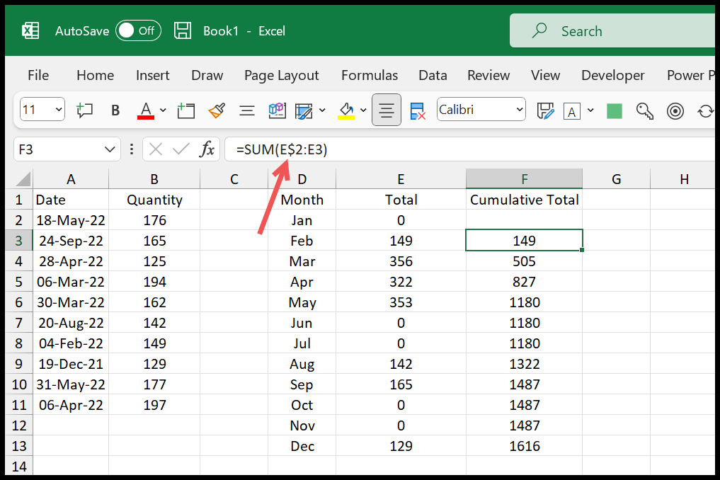
After that, drag the formula up to the last cell month.