

Click the chart title once to select it, type =, click the cell that holds the title text and press Enter. The formula bar shows a reference such as =Sheet1!$H$3, and the title changes whenever that cell does.
A chart title takes a single cell reference, not a formula. To mix fixed text with a value, build it in a helper cell, for example ="Monthly Sales Trend: "&H3, and link the title to that cell.
Wrap dates and numbers in TEXT, or the title shows the raw value, such as a date serial like 45658: ="Sales for "&TEXT(H3,"mmmm yyyy") or ="Total: "&TEXT(H4,"#,##0"). For a two-line title, join the parts with CHAR(10).
If = shows up as text in the title, you were editing inside the title rather than selecting it. Press Esc, check the title box is selected with no text cursor showing, then type = again.
The same link works on pivot chart titles and on text boxes or shapes: select the box, type = in the formula bar and click the cell. If the formula bar greys out when you select a title, as readers report on Box and Whisker charts, delete the title and lay a linked text box over the chart instead.
We all love dynamic and interactive charts. They are awesome. But, do you know what is the most important part of a dynamic chart?
That’s ➜ Chart Title
By creating a dynamic chart title, you can make your Excel charts more effective.
Just think this way. You have created a dynamic chart in which the values change when the current year changes. But what about the chart title? You need to change it every time.
The bad news is, there’s always a chance of missing it. But here is the good news: you can link a chart title with a cell to make it dynamic. And in today’s post, I’d like to share with you the exact steps to make a chart title dynamic by connecting it to a cell.
Let’s get started.
Steps to Create Dynamic Chart Title in Excel
Converting a normal chart title into a dynamic one is simple. But before that, you need a cell which you can link with the title.
Here are the steps:
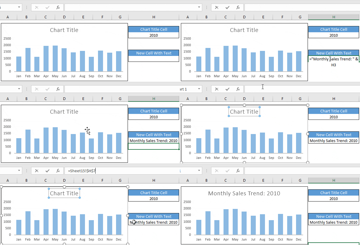
- Select the chart title in your chart.
- Go to the formula bar and type =.
- Select the cell which you want to link with the chart title.
- Hit Enter.
Excel puts the link in the formula bar with the sheet name, like =Sheet1!$H$3. From now on, the title shows whatever is in that cell.

Related: Top 10 ADVANCED Excel Charts and Graphs (Free Templates Download)
Combine Cell Links and Text to Create a Dynamic Chart Title
Now, let me show you how to combine a cell and a text to create a dynamic chart title. For example, let’s say you want to link a cell with a year that changes with the chart data, and you want to add the label “Monthly Sales Trend:” before it.
- First of all, just enter the formula below this list in a new cell, using the formula bar.
- Select the chart title.
- Go to the formula bar and type =.
- Now, just select the new cell.
- Hit Enter.
="Monthly Sales Trend: "&H3
Make sure to use straight quotes in the formula. If you copy a formula with curly quotes (“ ”), Excel shows an error instead of the title text.
If the cell has a date or a big number, wrap it in TEXT, or the title shows the date as a serial number (like 45731) and the number without separators:
="Sales as of "&TEXT(B1,"dd-mmm-yyyy")
Creating Dynamic Title in Pivot Chart
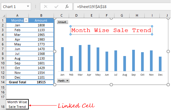
You can also use the same method to create a dynamic title in a pivot chart. Once you create a pivot chart, use the same steps as you have used in a normal chart.
Create a Dynamic Chart Title with Shapes
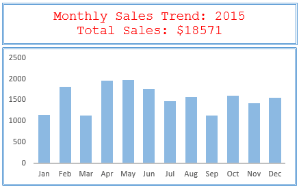
If you want to save some space in your chart, then you can also use a separate rectangular shape as a chart title.
- Just insert a shape into your worksheet.
- Select the shape, type = in the formula bar, select the cell and hit Enter, just as you linked the cell to the normal chart title.
Important Points
- You can’t use a formula in a chart title, but you can link it with a cell that has a formula.
- If you want to enter a line break in the chart title, you can create that line break in the cell you are linking to (Alt + Enter, or CHAR(10) in a formula).
- The same method works for axis titles and data labels: select them, type = in the formula bar and pick a cell.
Sample File
Download sample file from here to learn more.
Conclusion
A dynamic chart title depends on a cell that has a formula, which changes when the values in your chart change. So basically, your chart title is linked to a cell which is dynamic. I hope this charting tip will help you create advanced charts, and now tell me one thing.
Have you ever used a dynamic title in a chart before?
Share your views with me in the comment section; I’d love to hear from you. And please don’t forget to share this tip with your friends.
Frequently Asked Questions
Why does my chart title not update?
You probably typed the text into the title instead of linking it. Select the title and check the formula bar: a linked title shows a reference like =Sheet1!$H$3. If it doesn’t, link it again.
Can I link a chart title to a cell on another sheet?
Yes. After typing = in the formula bar, go to the other sheet, click the cell and hit Enter. Excel adds the sheet name to the link for you.
Can I type a formula directly into the chart title?
No. A chart title can only link to a single cell. Put the formula in a cell (it can be on a hidden helper sheet) and link the title to that cell.
More Charting Tips and Tutorials
- How to Add a Horizontal Line in a Chart in Excel
- How to Add a Vertical Line in a Chart in Excel
- How to Create a Bullet Chart in Excel
- How to Create a Dynamic Chart Range in Excel
- How to Create a Sales Funnel Chart in Excel
- How to Create a HEAT MAP in Excel
- How to Create a HISTOGRAM in Excel
- How to Create a Pictograph in Excel
- How to Create a Milestone Chart in Excel
- How to Insert a People Graph in Excel
- How to Create a Population Pyramid Chart in Excel
- How to Create a SPEEDOMETER Chart [Gauge] in Excel
- How to Create a Step Chart in Excel
- How to Create a Thermometer Chart in Excel
- How to Create a Tornado Chart in Excel
- How to Create Waffle Chart in Excel
Sr, please share, how to create dynamic chart of this tutorial…
I want to create a dynamic pivot chart title to describe the count of part-time & full-time and male & female hires (horizontal axis) along with the Month, Quarter, or Year (vertical axis) for drill downs. Is that possible?
Wow – no idea that it would be so simple. I have used Excel for 20 years in my career and for some reason never knew I could put a formula in as the Title. What a blessing you are to share such a simple task and educate us.
your words are blessings too. 🙂
Linking the title to a cell works for scatter plots and histograms, but I can’t get it to work with boxplots. Selecting the title in a boxplot deactivates the formula bar. Bummer.
You just saved me a lot of time and prevented a lot of mistakes!! Thanks!!
I’ve tried this countless times and researched to see if there was more to it, but like always I have failed. I am not sure why but every time I click on the chart title, the formula bar goes off. I need help!
Great, thanks
it is in excel sheet your sample file but cannot see the chart bar changing even though it is downloaded correctly, we have to convert to see , where we can see the bar change
Linking to a cell with a formula is a nice workaround for lack of direct formula in the title. Good one.
Thanks for your words Dinesh