

In Excel 2019, Excel 2021 or Microsoft 365, select your stage names and values, then go to Insert → Recommended Charts → All Charts → Funnel. The chart draws the stages in the order they sit on the sheet, so sort them largest first before you insert it.
In Excel 2016 or earlier, build it from a stacked bar chart. With stage names in column A and values in C2:C6, enter =(MAX($C$2:$C$6)-C2)/2 in B2 and fill it down. Select A1:C6, go to Insert → Charts and pick Stacked Bar. The helper is half the gap between each stage and the largest one, which pushes every bar in far enough to centre it.
Then make three changes. Right-click the vertical axis, choose Format Axis and tick Categories in reverse order so the first stage sits at the top. Click the helper bars and set Fill & Line → Fill → No fill. Click the value bars and set Series Options → Gap Width to 0% for a solid funnel, or around 10% to leave a gap between stages.
For an in-cell version with no chart, enter =REPT("|",C2/2) in a blank column, fill it down and centre the text. Large values make bars far wider than the cell, so scale to the biggest stage instead: =REPT("|",C2/MAX($C$2:$C$6)*50) gives the top stage 50 characters.
If the bars line up on the left instead of centring, the helper is being plotted after the values. Right-click the chart, choose Select Data and move the helper series to the top of the list.
The best way for you to track your sales is to use a funnel chart. A sales funnel chart not only describes the stages of the process but also provides a conversion funnel for your new business.

In today’s post, I’m going to show you the exact steps that you can use to create a sales funnel chart in Excel. And not just for sales, you can use this funnel chart for any process.
And now, let’s get started.
Steps To Create a Sales Funnel Chart in Excel
You have the following data table for this chart template which you can download from here to follow along.

- First of all, insert a dummy data column.
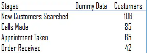
- In cell B2, insert the below formula into the formula bar and drag it down.
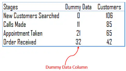 =(MAX($I$4:$I$7)-I4)/2
- To set up the sales funnel, just select the data and insert a stacked bar chart.
- Now, you have a chart like this.
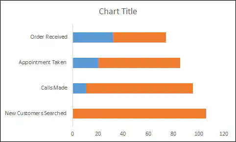
- From here, we need the following customization to transform this chart into a sales funnel chart.
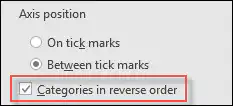
- Now, select the vertical axis and put the categories in reverse order. Format Axis → Axis Options → Categories in reverse order.
- After that, select the data bars for the dummy data and remove the fill color and border from them.
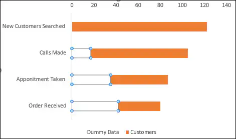
- In the end, select the data bars and change the gap width to 0%. Format Data Series → Series Options → Gap Width.
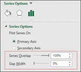
- And now, you have a neat and clean funnel chart to use as a template.
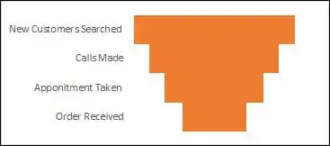
Congratulations! You made it.
Here’s the dummy column formula again so you can copy it. It takes half of the difference between the largest value and the value in that row, which pushes each bar to the center:
=(MAX($I$4:$I$7)-I4)/2
Change $I$4:$I$7 and I4 to the range and the first cell of your own values. For the largest stage, the formula returns 0, and for smaller stages, it returns a bigger gap, so the bars line up as a funnel.
Use the Built-in Funnel Chart
If you use Excel 2021, Excel 2024 or Microsoft 365, you don’t need the dummy column at all. Excel has a funnel chart type built in:
- First of all, select the stage names and their values (without the dummy column).
- After that, go to Insert ➜ Insert Waterfall, Funnel, Stock, Surface or Radar Chart ➜ Funnel. On a Mac, go to Insert ➜ Waterfall icon ➜ Funnel.
- In the end, format the bars and the data labels the way you like.
The built-in chart centers the bars on its own and shows the values as data labels. But if you share the file with someone on an older version of Excel, they won’t be able to see the chart, so the stacked bar method above is still useful.
Show the Conversion Rate in the Funnel
A funnel is more useful when you can see how many leads move from one stage to the next. Add a column next to your values with the following formula, format it as a percentage, and use it as the data labels (or show it next to the chart):
=I5/I4
This gives the conversion from the previous stage. To get the conversion from the first stage instead, lock the first value with =I5/$I$4.
[Bonus Tip] Funnel Chart Using REPT Function
As I earlier said, I’m a big fan of in-cell charting. Let me show you how to use the REPT function to create a sales funnel template in Excel. Creating an in-cell sales funnel chart is simple and quick; here are the steps.
- Take data in a simple form.
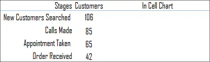
- In the blank column, enter the formula below and drag it down.
=REPT(“|”,D4/2)
- And now, change the text alignment of the bars to the center.
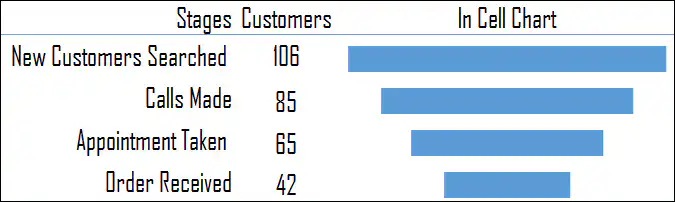
Your in-cell funnel chart is ready.
Here’s the formula to copy. REPT repeats the “|” character as many times as the value in D4 divided by 2, so a bigger value gives a longer bar. Change the 2 to make the bars shorter or longer:
=REPT("|",D4/2)
Download Sales Funnel Template
Conclusion
Using a sales funnel chart is one of the best ways of tracking a sales process. You can also add additional things in a chart as well, like conversion rate, pending percentage, etc.
All the steps which you have used above are simple and easy to follow. And, if you don’t want to put in the effort, you can go with the in-cell version.
I hope this tip helps you to get better at charting.
Now tell me one thing. Which method do you like the most?
And, if you have any other method to create a funnel chart, please share it with me in the comment box, I’d love to hear from you.
Please don’t forget to share this tip with your friends.
Frequently Asked Questions
Which Excel versions have a funnel chart?
Microsoft lists the built-in funnel chart for Excel 2021, Excel 2024 and Microsoft 365, on Windows and Mac. In older versions, use the stacked bar method from this tutorial.
Why are my funnel stages upside down?
A bar chart plots the first row at the bottom. Select the vertical axis and tick Categories in reverse order (Format Axis ➜ Axis Options) so the first stage is at the top.
Why is my funnel not centered?
The dummy column must come before the values column in the data, so it’s the first series in the stacked bar, and its formula must use the largest value of all the stages. Also, make sure the dummy bars have No Fill and not just a white color.
It says enter formula =(MAX($I$4:$I$7)-I4)/2 – but that makes no sense at all.
I have the same question here.
Hello Sir, really this helps a lot in our day today work. I didn’t understand like how to change the color of the each chart and how to insert the buttons as you did (Q1, Q2, Q3, Q4) Can you please help me with that
In-cell chart approach is so simple and elegant. Thanks for sharing. I am yet to understand the purpose of ‘divide by 2’ in the formula. I will keep thinking.
Hey Indzara, It’s nice you found it useful.
Dividing by 2 is just a matter to decrease the width of the bar.
Got it. That’s what I thought. May be it could be a formula based on the range of data instead of ‘2’, Either way, very good tip.
Thanks Dinesh for your words.
Cheers,
PG