

Add a helper column next to your data, label it Line, and type 100 only in the row where the line should sit, leaving the rest of the column empty. Select the whole table, including the helper column, and go to Insert → Insert Line or Area Chart → Line with Markers.
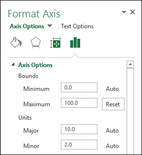
Right-click the helper series, choose Change Series Chart Type, set it to Clustered Column and tick Secondary Axis. Then right-click the secondary axis, choose Format Axis, and type 0 in Bounds → Minimum and 100 in Bounds → Maximum, so the column runs the full height of the plot area.
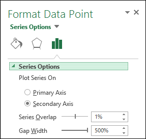
Hide that axis with Labels → Label Position → None, then select the column and raise Format Data Series → Gap Width to 500% to thin it into a line. To move the line, type the 100 in a different row.
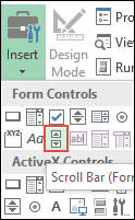
For a line you move with a scroll bar, turn on the Developer tab (File → Options → Customize Ribbon), add Developer → Insert → Scroll Bar (Form Control), right-click it, choose Format Control and link it to an empty cell outside the table, such as E1, with the maximum set to your number of rows. Replace the typed 100 with =IF(ROWS($A$2:$A2)=$E$1,100,"") in the first helper cell and fill it down.
If that formula returns #NAME?, retype the quotes: curly quotes copied from a web page are not read as an empty string. Keep the secondary axis bounds fixed rather than on Auto, too. That also keeps the line full height when your main data includes negative values, because the secondary axis scales separately from the primary one.
Sometimes, while presenting data with an Excel chart, we need to highlight a specific point to get the user’s attention there. And a simple way to do this is to add a vertical line to the chart.
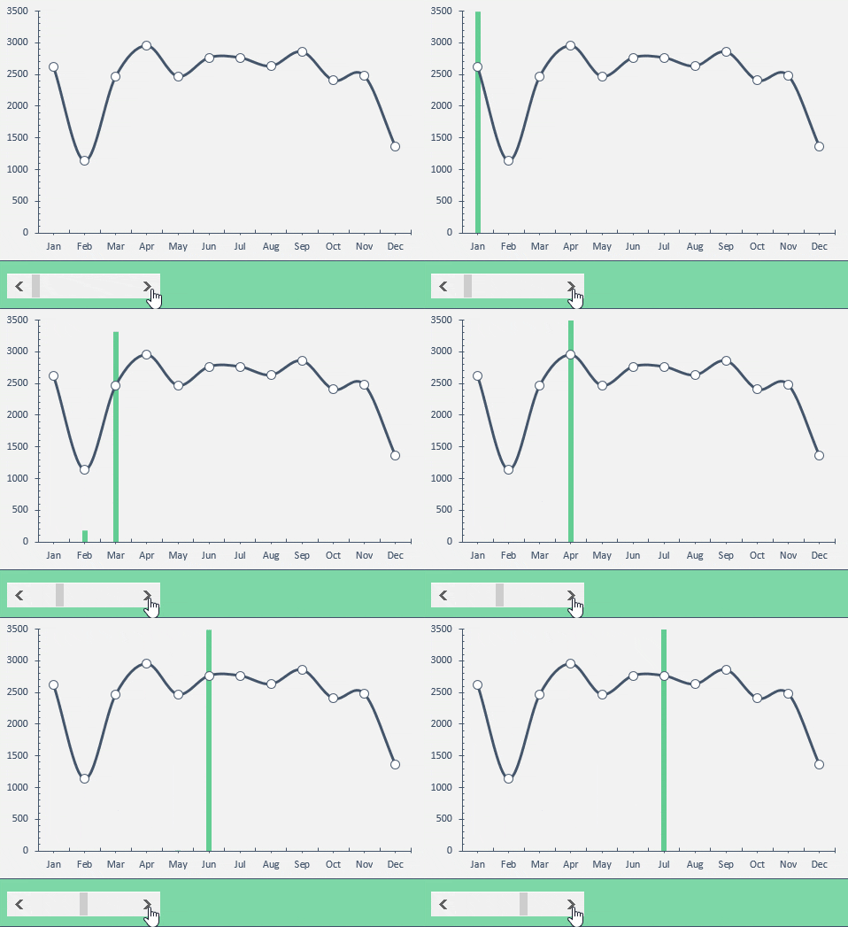
Yes, you heard it right. You can highlight a specific point on a chart with a vertical line. Just look at the below line chart with 12 months of data.
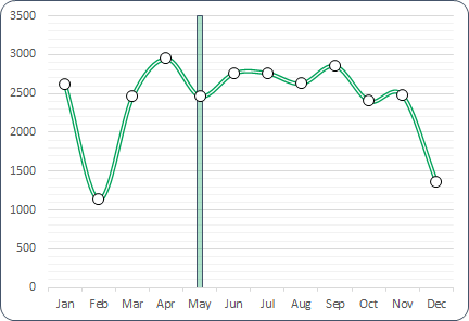
Now, you know the benefit of inserting a vertical line in a chart. But the point is, which is the best method? Well, out of all the methods, I’ve found this method (which I have mentioned here) simple and easy.
Without any further ado, here are the steps, and please download this sample file from here to follow along.
Steps to Insert a [Static] Vertical Line in a Chart
Here you have a data table with monthly sales quantity and you need to create a line chart and insert a vertical line in it. Please follow these steps.
- Enter a new column beside your quantity column and name it “Ver Line”.
- Now enter a value “100” for Jan in “Ver Line” column.

- Select the entire table and insert a line chart with markers.

- You’ll get a chart like this.

- Now select the chart and open the “Change Chart Type” options from the Chart Design tab.
- After that, for the “Ver Line” series, change the chart type to “Clustered Column” and tick the secondary axis box.

- The next thing is to adjust the axis values for your column bar.
- Double-click on your secondary axis to open the formatting options.
- Under Bounds, change the Maximum value to 100, as we have entered the same value in the Ver Line column (keep the Minimum at 0).
- In the same axis options, move down to Labels ➜ Label Position and select None (this hides the secondary axis; yup, we don’t need it).

- Last but not least, we have to make our column bar a little thinner so that it looks like a line.
- Click on the data bar, go to Series Options and increase the “Gap Width” to 500% (the maximum).
Congratulations! You have successfully added a vertical line to your chart. You can download this sample file from here to learn more about this.
Quick Tip: Just enter 100 in the row of the month where you want the vertical line. If you want to move the line to another month (say Feb), delete the value and enter 100 in that month’s row instead.
Steps to Add a [Dynamic] Vertical Line in a Chart
Now it’s time to level up your chart and make a dynamic vertical line. Please follow these simple steps for this.
- First of all, you need to insert a scroll bar. Go to the Developer tab ➜ Insert ➜ Scroll Bar (Form Control).
- Right-click on your scroll bar and select Format Control.
- Link your scroll bar to cell D1 (the cell the formula below uses), enter 1 for the minimum value and 12 for the maximum value.

- In the end, click OK.
- After that go to your data table and insert this formula [=IF(MATCH($A2,$A$2:$A$13,0)=$D$1,100,””)] in cell C2 (Formula Bar) and drag down up to the last cell of the table.
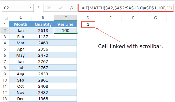
- Now you can use the scroll bar to navigate your vertical line in your chart. You can download this sample file from here to learn more about this.
Here’s the formula from step 5 to copy. It returns 100 only for the month whose position in the list matches the number in D1, and a blank for all other months:
=IF(MATCH($A2,$A$2:$A$13,0)=$D$1,100,"")
Add a Vertical Line for the Current Month
If you want the line to move on its own to the current month, you don’t need a scroll bar. When the months in column A are short names like Jan and Feb, use this formula in the Ver Line column instead:
=IF(A2=TEXT(TODAY(),"mmm"),100,"")
Every time the workbook recalculates, the line moves to the month of today’s date. Note that TEXT returns the month name in your Excel language, so the names in column A need to match it.
Add a Label to the Vertical Line
To tell the reader why the line is there, add a label to it. Click the column bar, then right-click and select Add Data Labels. After that, right-click the label, select Format Data Labels, and under Label Options, tick Value From Cells and select a cell with your text (like “Launch”). Untick Value so only your text shows.
Conclusion
As I said, adding a vertical line in a chart is useful when you want to highlight a specific data point in your chart. There are also some other ways to add a vertical line, but I found this method quick and easy. I hope this charting tip will help you to get better at Excel.
Have you ever tried to do this before with your chart?
Please share your views in the comment section. I would love to hear from you, and please don’t forget to share this tip with your friends.
Frequently Asked Questions
Why is my vertical line not reaching the top of the chart?
The secondary axis maximum isn’t fixed at the value you entered. Set the Maximum bound of the secondary axis to 100 (the same value as in the Ver Line column), and the column fills the full height.
Can I change the color of the vertical line?
Yes. Right-click the column bar, select Format Data Series, and change the Fill color. A bright or dark color makes the line stand out from the data line.
Does this work with a column chart?
Yes, but the line column sits next to the data columns. To keep it on top, make sure it’s on the secondary axis, as in the steps above, so it’s drawn over the main columns.
More Charting Tips and Tutorials
- How to Add a Horizontal Line in a Chart in Excel
- How to Create a Bullet Chart in Excel
- How to Create a Dynamic Chart Range in Excel
- How to Create a Dynamic Chart Title in Excel
- How to Create Interactive Charts In Excel
- How to Create a Sales Funnel Chart in Excel
- How to Create a HEAT MAP in Excel
- How to Create a HISTOGRAM in Excel
- How to Create a Pictograph in Excel
- How to Create a Milestone Chart in Excel
- How to Insert a People Graph in Excel
- How to Create PIVOT CHART in Excel
- How to Create a Population Pyramid Chart in Excel
- How to Create a SPEEDOMETER Chart [Gauge] in Excel
- How to Create a Step Chart in Excel
- How to Create a Thermometer Chart in Excel
- How to Create a Tornado Chart in Excel
- How to Create Waffle Chart in Excel
Amazing tutorial. I learned a lot from it!
Great tutorial! Many thanks for your contributions!
Thanks a lot. This method works better and faster. More than that, I love the comment section of your articles because the answers provided gives me an added lesson that I would one day live to confront and them solve.
Thanks again
very interesting and informative..thankyou for posting this
I try to drag the formula in C2 to add dynamic vertical line.But in the cell the message come as #Name ?.Pl help
Try it with the sample file.
Puneet you may not see this but thank you this worked great.
I’m so glad you liked it. 🙂
Hi, I’ve had a play with this and the concept makes a lot of sense. This is handy. However, I’ve now got another issue for mine.
What if my graph also includes negative values? This works well when all values are positive, but my graph actually includes negatives! Thanks in advance.
This solution works for the dynamic version of the chart:
In that case, I believe you should have a condition if the value in the selected cell (which you are selecting with a scroll bar) has a negative value then the value for the vertical line also be negative.
Ingenious and Intersting!
I could have used it had I known it a year earlier! When I was updating numerous charts on a weekly basis to depict various facets of my project. My X-Axis was always fixed to span entire 18 month project life span. And I was using an actual vertical line to depict the Status Date and would move it physically on all the charts. The scroll button would have been more professional!
Is it possible to move the line on multiple charts using the same scroll button?
Yes you can. Let’s say if you have 1 to 12 scroll bar numbers for the first chart then you can use 13 to 24 for the second chart.
Thanks’ I make use of this.
Welcome.
I’m so glad you found this post helpful!
Thanks Puneet, nice sharing and I second your statement it is an easy method.
Hey Asif,
Thanks for your words.