

AutoFormat is hidden in current Excel, so add it first: open File → Options → Quick Access Toolbar, set Choose commands from to Commands Not in the Ribbon, select AutoFormat, then click Add and OK.
Click any cell in your data, click the AutoFormat button and pick one of the 16 designs. Click Options to choose which parts it applies (number format, font, alignment, border, patterns, width/height); untick Width/Height to keep your column widths.
For most tables, Home → Format as Table (or Ctrl + T) is the better choice. Table styles extend to new rows automatically and add filters and banded rows, while AutoFormat applies fixed formatting that new rows don’t pick up.
To undo AutoFormat, choose None at the end of the AutoFormat list, or select the data and press Alt → H → E → F to clear all formatting.
If you want to stop Excel changing things as you type, such as turning web addresses into links, that’s a different setting: File → Options → Proofing → AutoCorrect Options → AutoFormat As You Type.
Formatting is a tedious task. It’s really hard to format your data whenever you present it to someone. But this is the thing that makes your data more meaningful and easy to consume.
It would be great if you have an option that you can use to format your data without spending much time. So, when it comes to Excel, you have an amazing option that can help you to format your data in no time.
Its name is AUTO FORMAT. In auto-format, you have several pre-designed formats which you can apply to your data instantly.
All you have to do is select a format and click OK to apply it. It’s simple and easy. In all the pre-designed formats you have all the important components of formatting, like:
- Number Formatting
- Borders
- Font Style
- Patterns and Background Color
- Text Alignment
- Column and Row Size
In this post, you will learn about this amazing option that can help you to save a ton of time in the coming days.
Quick Note: It’s one of those Excel Tricks that can help to get better at Basic Excel Skills. So, let’s get started…
Where to Find the AUTO FORMAT Option?
If you check the Excel 2003 version, the auto-format option is there on the Format menu. But, with the release of Excel 2007 and the ribbon, this option is not available on any of the tabs.
That doesn’t mean you can’t use it in later versions. It’s still there but hidden. So, to use it in Excel 2007 and later versions (including Excel 2016, 2019, 2021 and Microsoft 365), you need to add it to your Excel’s quick-access toolbar. It’s a one-time setup so you don’t have to do it again and again.
Add Auto Format on the Quick Access Toolbar
To add the auto format to your quick access toolbar please follow these steps.
- First of all, go to your quick access toolbar and click on the small down arrow at the end of the toolbar.
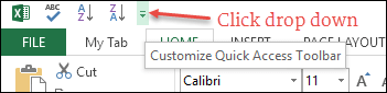
- And, when you click on it, you will get a drop-down menu.
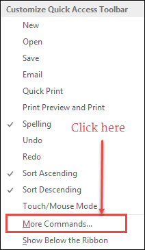
- From this menu, click on “More Commands”.
- Once you click on it, it will open “Customize the Quick Access Toolbar” in the Excel options.
- From here, click on the “Choose commands from” drop-down and select “Commands Not in the Ribbon”.
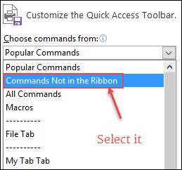
- After that, come to the list of commands you have right below this drop-down.
- And, select the “AutoFormat” option and click Add to add it to the quick access toolbar.
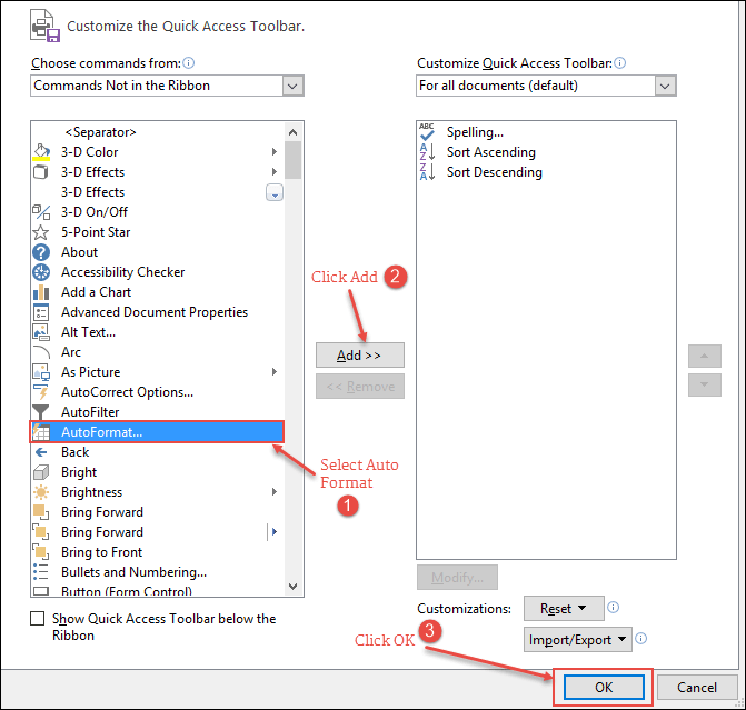
- Click OK.
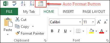
Now, you have the auto-format icon in your quick-access toolbar.
How to Use Auto Format?
Applying formats with an auto-format option is super simple. Let’s say you want to format the below data table.
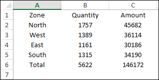
Download this file from here to follow along and follow the below steps to format the table.
- Select any of the cells from your data.
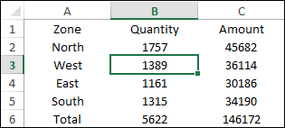
- Go to the quick access toolbar and click on the auto-format button.
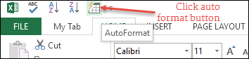
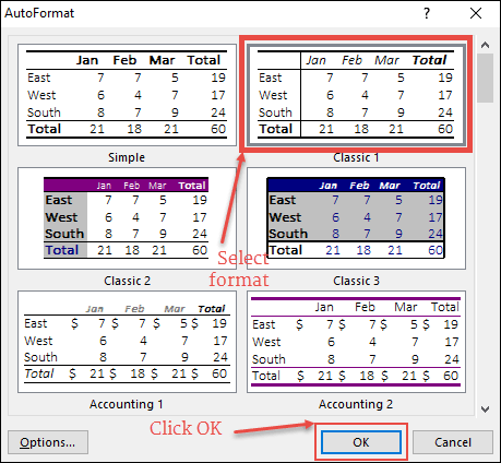
- Now, you have a window where you have different data formats.
- Select one of them and click OK.
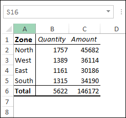
- Once you click OK, it will instantly apply your chosen format to the data.
How to Modify a Format in Auto Format
As I mentioned above, all the formats in the auto format are a combination of 6 different components. And you can also add or remove these components from each format before applying them.
Let’s say, you want to add formatting to the below data table but without changing its font style and column width. You need to apply the format using the below steps.
- Select your data and click on the auto-format button.
- Select a format to apply and click on the “Options” button.
- From options, un-tick “Font” and “Width/Height”.

- And, click OK.

Now, neither of these components is part of your formatting.
Removing Formatting
Well, to remove formatting from data, the best way is to use the shortcut key Alt + H + E + F (Home ➜ Clear ➜ Clear Formats). But you can also use the auto format option to remove formatting from your data.
- Select your entire data and open auto format.
- Go to the end of the format list, where you have a “None” format.

- Select it and click OK.
Important Points
- AutoFormat doesn’t check if you already have some formatting on your data. It ignores it and applies new formatting as per the format you have selected (for the components that are ticked in Options).
- You need at least 2 cells to apply formatting with the auto-format option.
- AutoFormat works on the whole data range around the active cell (the current region), so leave a blank row and column between separate tables.
Auto Format vs Format as Table
In newer versions of Excel, Microsoft’s own replacement for AutoFormat is Format as Table (Home ➜ Format as Table, or Ctrl + T). Here’s how they compare:
- Auto Format: applies fixed formatting to the cells. If you add a new row later, it isn’t formatted, and you need to apply the format again.
- Format as Table: turns the range into an Excel table, so new rows get the same style on their own, and you also get filters, banded rows and structured references.
- Cell Styles: on the Home tab, these apply a saved set of formats to single cells, like headings or totals.
Apply Auto Format with VBA
You can also apply an AutoFormat with a macro, using the AutoFormat method of a range. The following code applies the “Classic 1” format to the data around cell A1, without changing the font and the column widths:
Sub ApplyAutoFormat()
    Range("A1").CurrentRegion.AutoFormat _
        Format:=xlRangeAutoFormatClassic1, _
        Font:=False, Width:=False
End Sub
Frequently Asked Questions
Is AutoFormat available in Excel 365?
Yes, in Excel for Windows. It isn’t on the ribbon, but you can add it to the quick access toolbar from “Commands Not in the Ribbon”, as shown above.
Why does AutoFormat format more cells than I selected?
When you select a single cell, AutoFormat picks the whole data range around it. Select the exact range first if you only want to format part of the data.
Can I undo AutoFormat?
Yes. Press Ctrl + Z right after applying it, or apply the “None” format from the AutoFormat list later.
Thank you so much!
Welcome
Very useful and very good narration.
yes ofcourse auto-formating is a very good thing . it gives instant designs and also saves the time.
Time Saver Hacks 🙂
Very useful for accountants
Im a little confused. Why is Auto format is used for, and why is it important?
quick formatting.
Thank you Puneet for the answer
🙂
Brilliant !!
Hey Zahid, Thnaks for your words.