Highlight Alternate Rows in Excel with Color Shade

In Excel, when you are working with a large set of data, in that case, to have better look and increase the readability, you can highlight alternate rows with a color shade. It makes each row of the data distinct and helps you to read it.

In this tutorial, we are going to discuss three simple ways that you can use.

Use an Excel Table to Highlight Alternate Rows in Excel

Using an Excel table is the best as well as the easiest way to get apply a shade of color to highlight alternate rows in Excel.

1. Select the data on which you want to apply it.
   
2. After that, go to the Insert Tab, and click on the table button. You can also use the keyboard shortcut Control + T.
   
3. Now, from the dialog box, make sure to check to mark “My table has headers”.
   
4. In the end, click OK to apply the table.

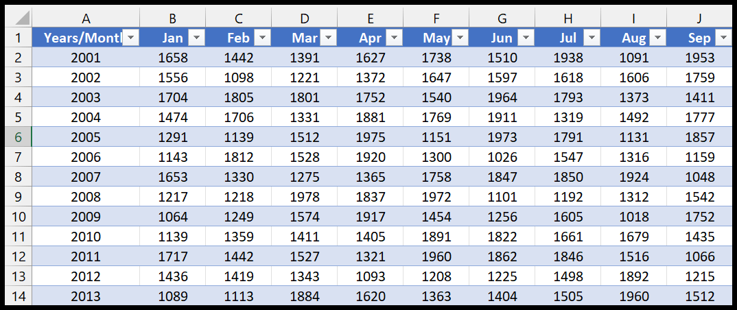
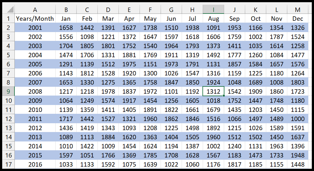
Once you click OK, you will get a default table style on your data, just like the following.

But you can change the style if you don’t want to go with the default one. Go to the Table Design Tab, and then open the Table Styles.

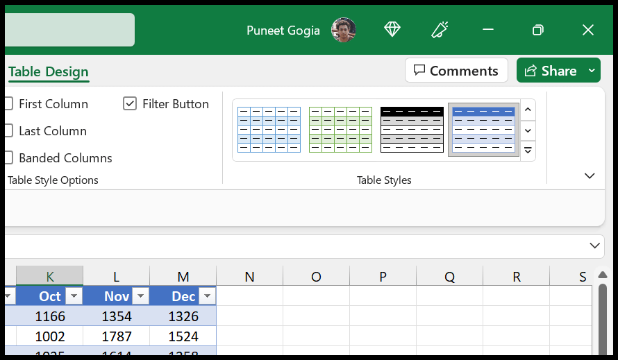
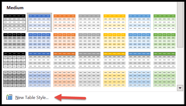
From the styles, you can choose one or you can create a style for yourself from the scratch.

Using Conditional Formatting to Apply Color Shades on Alternate Rows

You can also use a formula in the conditional formatting to apply a shade of color to each row that you have in the date. This method gives you better control you can have a more customized way.

1. First, select the data on which you want to apply the color shades.
   
2. After that, go to the Home Tab and click on the conditional formatting Drop Down.
   
3. From there, click on the New Rule.
   
4. Next, click on “Use a formula to determine which cell to format”.
   
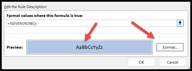
5. At this point, you have an input bar to add a formula, just like I have below.
   

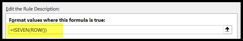
Now, you need to enter one of the below formulas:

• =ISEVEN(ROW()) – If you want to shade the even rows.
• =ISODD(ROW()) – If you want to shade the odd rows.

After that, click on the format button to decide which color shade you want to give to each alternate row to highlight it.

In the end, click OK to apply the conditional formatting.

Use a VBA code to Apply a Color to Alternate Rows

You know how to use VBA in Excel; you can use a macro to apply a color shade to each alternate row. Just select the range and run the following code.

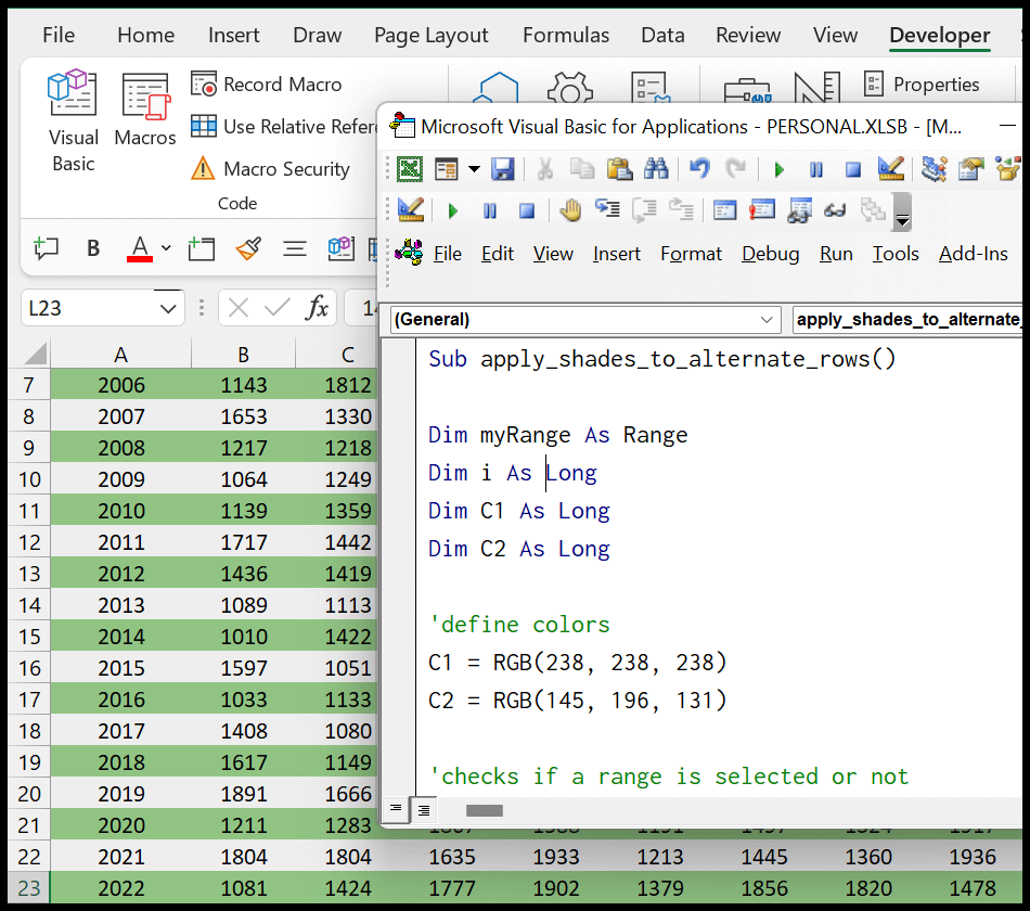
Sub apply_shades_to_alternate_rows()

Dim myRange As Range
Dim i As Long
Dim C1 As Long
Dim C2 As Long

'define colors
C1 = RGB(238, 238, 238)
C2 = RGB(145, 196, 131)

'checks if a range is selected or not
If TypeName(Selection) <> "Range" Then Exit Sub

'specify the range to the variable
Set myRange = Selection

'end the code if only one row is selected
If myRange.Rows.Count = 1 Then Exit Sub

'loop through each row one by one and color alternate rows with different color shade
  For i = 1 To myRange.Rows.Count
    If i Mod 2 = 0 Then
      myRange.Rows(i).Interior.Color = C2 'Even Row Shade
    Else
      myRange.Rows(i).Interior.Color = C1 'Odd Row Shade
    End If
  Next i

End Sub

Quick Links: Visual Basic Editor – Run a VBA Code