

To average a range while ignoring zeros, use =AVERAGEIF(A1:A10,">0"). The criteria goes inside double quotes, and you can leave the third argument out — when you skip it, AVERAGEIF averages the same range it’s testing.
AVERAGE already ignores blank cells and text, but it treats a zero as a real value, which is why a column with several zeros pulls the average down. Note that ">0" also excludes negative numbers, so if your data can go below zero use =AVERAGEIF(A1:A10,"<>0") instead — that excludes only the zeros.
To average non-zero values that also meet another condition, switch to AVERAGEIFS: =AVERAGEIFS(B1:B10,B1:B10,"<>0",A1:A10,"North"). One thing to watch: if every value in the range is zero, there’s nothing left to average and the formula returns #DIV/0! — wrap it in =IFERROR(AVERAGEIF(A1:A10,"<>0"),0) if that’s possible in your data.
When you average values in Excel, you can write a formula in a way to exclude or ignore cells with a zero. In this tutorial, we will look at the way to write this average formula.

Ignore Zero while Averaging Values in Excel
You can use the below steps:
- First, enter the function AVERAGEIF in a cell.
- After that, in the first argument, refer to the range where you have values.
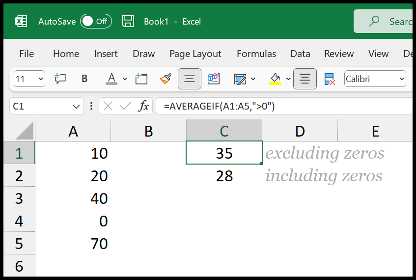
- Now, in the second argument, enter “>0”. This tells Excel to only include values greater than zero.
- In the end, enter closing parentheses and hit enter to get the result.

You don’t need to specify the average_range, which is an optional argument. When you skip specifying it, AVERAGEIF average values from the range that you specify in the range criteria.
Below you can see the difference between the average result when you exclude zeros and when you include zeros.
Written by
Puneet Gogia
Microsoft MVP — Excel · Founder, Excel Champs
Twelve years of teaching Excel, and a decade before that using it as a data analyst. Every tutorial here is written from a file I actually built.