

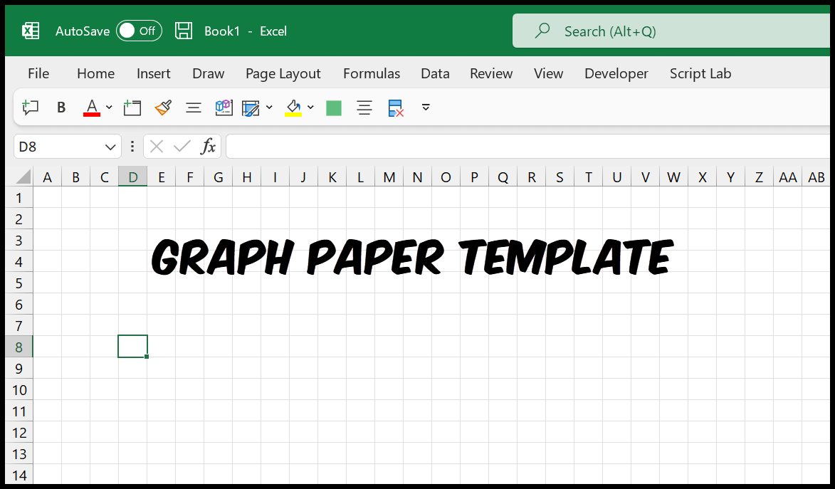
In Excel, you can create graph paper and take a printout of it for later use. In this tutorial, we will learn to make this template using simple and easy-to-follow steps. In this graph paper template, you will have small square boxes (with the same height and width).
Create a Graph Paper in Excel
- First, click on the Select All button at the top-left corner of the worksheet, or you can use the keyboard shortcut Ctrl + A to select all the cells.

- Go to the “Home” tab and in the Cells group, click on the Format drop-down.

- From here, click on the “Column Width” option.

- And in the Column Width box, enter “3” and then click OK to save.

- Now, you have graph paper-like boxes in your worksheet.

- Press the Ctrl + P to open the print preview and then click on “Page Setup”.

- Next, in Page Setup, go to the Margins tab, and make the header and footer 0, top, bottom, left, and right margins 0 or 0.5.

- Click on both checkboxes (Horizontal and vertical) under “Center on page”.

- Next, go to the “Sheet” tab in the Page Setup dialog, and under the “Print” group, tick the “Gridlines” checkbox to print the gridlines and click OK to save.

At this point, all the setup is done that you need to do, and the next thing is to print the graph paper.
A column width of 3 gives you narrow boxes, but they aren’t exact squares, as the default row height is 15 points (20 pixels). For true squares, set the column width to 2.14 (also 20 pixels), or set both the row height and the column width in the same unit from View ➜ Page Layout, where you can enter sizes in centimetres or inches (like 0.5 cm for both).
Print the Graph Paper in Excel
Even though we made all the settings, our sheet is still blank, and Excel will not print a blank sheet. So, we need to add empty spaces to one single page to make it work while printing.
- First, go to the View tab and click on the “Page Layout” button.

- Now, enter a space in the first cell and then copy and paste that space to the cells that you have on the single page.

- Go back to the “View” tab and click the “Normal” view button from there.

- In the end, go to File ➜ Print to see the print preview, or just use the shortcut key Ctrl + P to check the print preview.

And once you hit the Print button, you’ll get a printout of the graph paper just like above. You can also save a PDF file from your Excel workbook as well (File ⇢ Export ⇢ Create PDF/XPS Document ⇢ Create PDF/XPS).

Use Borders Instead of Gridlines
Another way, which doesn’t need the spaces, is to use borders. Select the range that fits on one page (for example, A1:AF55), and go to Home ➜ Borders ➜ All Borders. Cells with borders are printed even when they are empty, and you can also pick a lighter line color from Borders ➜ Line Color, so the grid looks like real graph paper.
Frequently Asked Questions
Why does Excel say “We didn’t find anything to print”?
Because the sheet is empty. Gridlines alone don’t count as content, so add the spaces as shown above, or use borders.
How do I print graph paper on more than one page?
Fill the spaces (or borders) over the cells of all the pages you want, or simply print the same page several times by changing the number of copies in the Print screen.
Can I save the graph paper as a template?
Yes. Go to File ➜ Save As and choose “Excel Template (*.xltx)” as the file type. Next time, open it from File ➜ New ➜ Personal.
Written by
Puneet Gogia
Microsoft MVP — Excel · Founder, Excel Champs
Twelve years of teaching Excel, and a decade before that using it as a data analyst. Every tutorial here is written from a file I actually built.