How to Count the Colored Cells in Excel

It is very common to use cell colors to mark some cells as important or different from others, right?

Let us say you are managing a project and using Excel to track the status of different tasks. You have a list of tasks in column A, and in column B, you mark each task as “Completed” or “In Progress”.

You have used different background colors to make it easier to check out the cells: green for completed tasks and yellow for tasks still in progress.

You need to quickly count how many tasks are completed by counting the green cells.

Though there are a lot of functions and formulas in Excel to count cells and rows, there’s no default function that can help you count the cells with a particular color. So, the only way is to count them manually.

However, instead of manually counting the colored cells, you can use a custom function, formula, or VBA code.

Key Points

• The best way to count cell colors is using a custom VBA code-created function.
• You can also use a GET.CELL function to write a formula to count the cells with color using a helper column.
• If you don’t need to count all the time, you can use SUBTOTAL and Filter to get the count of colored cells whenever you need.

In this tutorial, we will learn how to count the colored cells using the methods I have mentioned above. So, let’s get started…

Use a Custom Function to Count Colored Cells (VBA Code)

The best way to count the cells with color is to use a VBA code to create a custom function specifically designed to count the colored cells.

Look at the code below, which is written to count specific color cells. You can use this code to create this custom function.

Function CountColorCells(rng As Range, colorCell As Range) As Long
    Dim cell As Range
    Dim colorToCount As Long
    Dim count As Long
    
    ' Get the color index of the specified cell
    colorToCount = colorCell.Interior.Color
    
    ' Loop through each cell in the range
    For Each cell In rng
        If cell.Interior.Color = colorToCount Then
            count = count + 1
        End If
    Next cell
    
    ' Return the count
    CountColorCells = count
End Function

To understand how to use this code, you need to use these simple steps,

1. Press Alt + F11 to open the VBA editor.
2. Insert a new module (Insert > Module) and paste the above code.
3. Come back to your Excel worksheet.
4. Use the function like this:

=CountColorCells($A1:$A10,C1)

This custom function has two arguments to define: the range of cells you want to check (rng) and the cell whose cell color you want to compare (colorCell).

First, it determines the color of the cell you referred to in the second argument using the “.Interior.Color” property to get that cell’s background color code.

After that, it loops through each cell in the specified range and compares its background color to the color of the reference cell.

If a cell has the same color, the counter increases by one. Once it has checked all the cells, the function returns the total number of cells that match the color.

Read Also: Apply Background Color to a Cell / Keyboard Shortcut to Fill Color

In the same way, here is code that can help you create a custom function to count cells based on the font color.

Function CountFontColorCells(rng As Range, colorCell As Range) As Long
    Dim cell As Range
    Dim colorToCount As Long
    Dim count As Long
    
    ' Get the font color of the specified reference cell
    colorToCount = colorCell.Font.Color
    
    ' Loop through each cell in the range
    For Each cell In rng
        ' Check if the font color matches the reference cell's font color
        If cell.Font.Color = colorToCount Then
            count = count + 1
        End If
    Next cell
    
    ' Return the count
    CountFontColorCells = count
End Function

Now, this custom function takes the cell’s font color instead of the cell color. You need to refer to the range of cells and the cells where that font color is applied.

=CountFontColorCells($A$1:$A$10,C1)

This code also works like the above code, using a loop to loop through all the cells in the range and match the defined font color with the cell’s font color. If the font color matches, it counts that cell and adds it to the total count.

Here’s one more piece of code that helps you create a custom function that can count cells based on both font color and cell color.

=CountColorCellsAD($A$1:$A$10,C1,1)

Function CountColorCellsAD(rng As Range, colorCell As Range, Optional countType As Boolean = False) As Long
    Dim cell As Range
    Dim colorToCount As Long
    Dim count As Long
    
    ' Determine whether to count based on font color (1) or cell color (0)
    If countType = True Then
        colorToCount = colorCell.Font.Color ' Get the font color of the reference cell
    Else
        colorToCount = colorCell.Interior.Color ' Get the background color of the reference cell
    End If
    
    ' Loop through each cell in the range
    For Each cell In rng
        If countType = True Then
            ' Check if the font color matches the reference cell's font color
            If cell.Font.Color = colorToCount Then
                count = count + 1
            End If
        Else
            ' Check if the background color matches the reference cell's background color
            If cell.Interior.Color = colorToCount Then
                count = count + 1
            End If
        End If
    Next cell
    
    ' Return the count
    CountColorCellsAD = count
End Function

In the custom function, you have three arguments to define:

• rng: The range of cells you want to check.
• colorCell: The reference cell for color comparison.
• countType: A Boolean value where 0 counts based on cell color, and 1 counts based on font color. If you skip specifying the value, it counts based on the cell color.

Here is the code that creates a custom function that counts all the cells that have color.

Function CountAllColoredCells(rng As Range) As Long
    Dim cell As Range
    Dim count As Long
    
    ' Loop through each cell in the range
    For Each cell In rng
        ' Check if the cell has a background color
        If cell.Interior.ColorIndex <> -4142 Then ' -4142 is the code for "no fill"
            count = count + 1
        End If
    Next cell
    
    ' Return the count
    CountAllColoredCells = count
End Function

Count Cells Based on Cell Color without VBA (GET.CELL)

Yes, there’s a way that you can count the cells based on the cell color, and you do not need to count a VBA code for this.

In Excel, there is a VBA function named GET.CELL lets you extract specific information about a cell, such as its cell color, font color, or value.

This function is not in the list of Excel functions; it is only there for compatibility. You can use it to get a cell’s color.

Note – To use this function, you need to create a named range, a helper column, and the COUNTIF function to count the cells with color.

1. Create a Named Range
2. Add a Helper Column
3. Use COUNTIF to Count the Cells

1. Create a Named Range

So, let’s create a name range first. First, select cell A2. Then, go to the Formulas Tab and click on “Name Manager.” You can use this option to create a new name range.

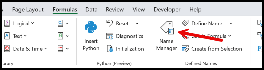
When you click the button, a dialog box opens to create a named range. In this dialog box, click on “New” to open a further dialog box to enter the details.

In the “New Name” dialog box, you need to click on enter a few details, like the following:

• Name: GetFontColor
• Scope: Workbook
• Refer to: =GET.CELL(38,Sheet2!A1)

Once you enter these details, you only need to click OK to save them and then click OK again to create the named range.

Now, let’s understand why this formula you used in the “Refer to” work works and why we can use it directly in the worksheet.

You need to understand that when we used A1 in the cell reference, we referred to the cell adjacent to cell A2, so we selected it before creating the named range. This way, whenever you use the named range in any of the formulas, it will refer to the adjacent cell from the left side and return its cell color code (38 in the code to get the cell’s color in return).

Read Also – Color Scales in Conditional Formatting/ Sort by Color in Excel/ Count Characters in Excel

2. Create a Helper Column

From here, the next step is to create a helper column to get the code of the cell color in the column. We need to use the named range we created using the GET for this.CELL.

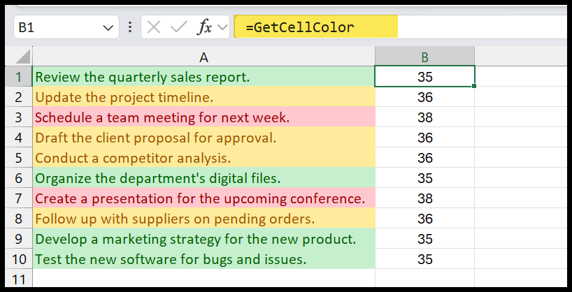
In the above example, we have entered “=GetCellColor” in cell B1. When you enter it in cell B2, it takes the information from the adjacent cell on the left side, that is, from cell A1.

That means you have the color code in cell B1 of the cell color you applied to cell A2.

3. Count Cells with Color

In the end, you need to use COUNTIF using the color code. We have a code for each color in the helper column, so we need to use COUNTIF, like the one in the following.

=COUNTIF($B$1:$B$10,GetCellColor)

Here, we have used the COUNTIF and referred to the helper column, which is the range “B1:B10.”
In the second argument, we have used the named range, which refers to the adjacent cell on the right side, to get the color code from there.

So here, COUNTIF, take the color code from the cell you refer to and then use the code and the count of cells from the helper column to give you a count of the cells for that particular color.

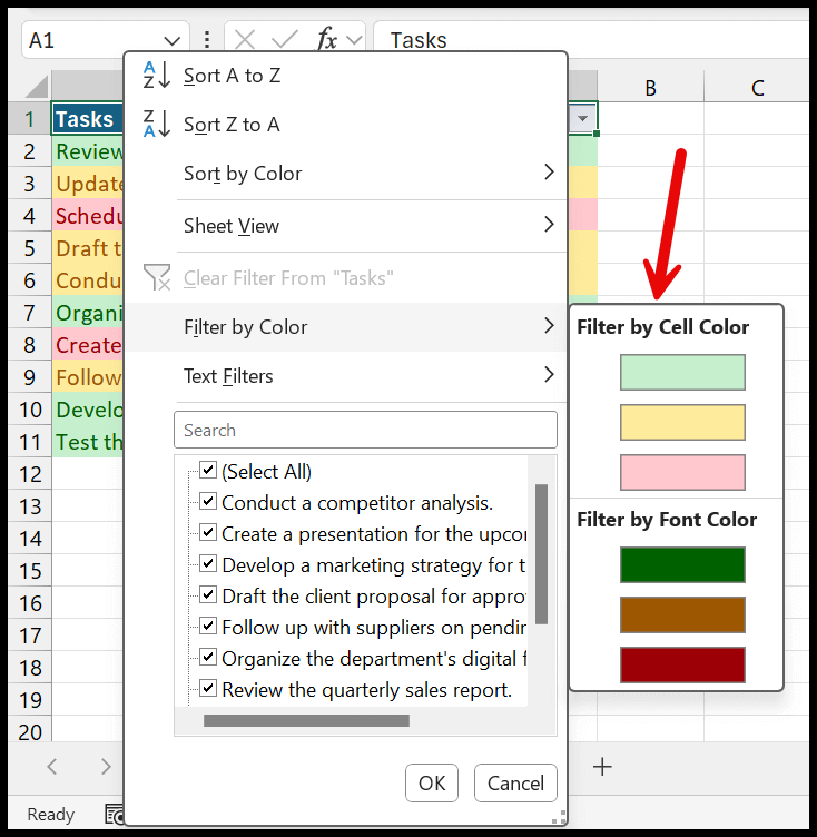
Count the Cells with a Particular Color using a Filter

You can count the cells in Excel based on the filter’s color. When you have colors applied to one cell in a column, when you open the filter, you can see the option “Filter by Color.”

Now, to count these cells with a color, you need to use the SUBTOTAL function, which allows you to count the cells dynamically. When you filter the column, you can use the formula below to get any cell count.

Read Also – Count Unique Values in Excel / COUNTIF – COUNIFS with OR / COUNTIF for Blank Cells Count in Excel

In the End

If you ask me which method is better than the other two, there is no such thing as which method is better.

The only difference is that you can use VBA and GET.CELL when you need to count the colored cells or cells based on the font color in real-time.

And if you need to know the count of the cells with color not so frequently when you can use the SUBTOTAL function with a Filter.

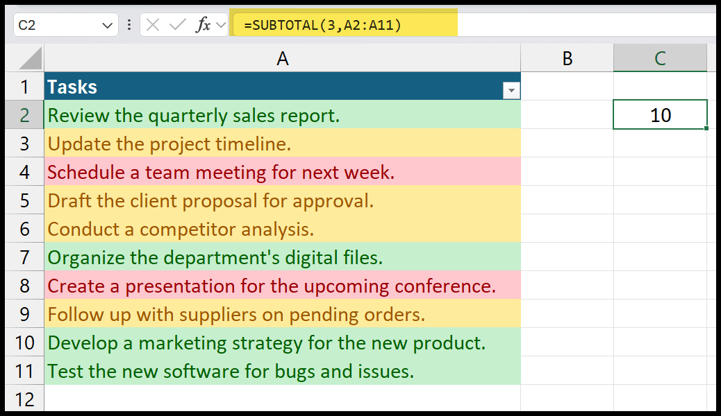
In Excel, SUBTOTAL calculates a range of data, such as sum, average, count, etc. It is unique because it can exclude filtered-out or hidden rows depending on the first argument.

In the first argument, we used three (3), which tells the function of counting all non-empty cells and ignoring the cells if any of the cells are filtered out. In the second argument, we have specified the range of cells we have colored cells.

Now, when you apply a filter for a color for which you want to count the cells, SUBTOTAL works.

In the above example, we have filtered cells with the green cell color, and subtotal has returned the count of the cells in the result.

If you want to count cells or any other cells, you can filter cells with that color. You can filter cells based on the font color instead of the cell color, and SUBTOTAL will also count those cells for you.