

Select the range, then go to Home → Conditional Formatting → Color Scales and click one of the 12 preset scales. Hover over a scale to preview it on your data first. With Green – Yellow – Red, the highest values turn green and the lowest turn red.
To choose your own colors or thresholds, go to Home → Conditional Formatting → Color Scales → More Rules, pick 2-Color Scale or 3-Color Scale under Format Style, and set the Type for each point: Lowest/Highest Value, Number, Percent, Percentile or Formula. For scores out of 100, use Number with 0 and 100 so the colors stay put when the data changes.
The Formula type sets a threshold, not the rule. Enter =AVERAGE($B$2:$B$20) as the Midpoint to centre the scale on the average. Each cell is still colored by its own value.
Excel has no 4-colour or 5-colour scale. For more bands, add one rule per band with Home → Conditional Formatting → New Rule → Format only cells that contain, set Cell Value between (for example 2000 and 3999), and give each rule its own fill. You get solid bands rather than a gradient.
If some cells stay uncolored, they hold numbers stored as text or are blank, and color scales skip both. Select them, click the warning icon and choose Convert to Number. To show only the colors, press Ctrl + 1, choose Custom and type ;;; to hide the values.
What is the Color Scales Option?
Color Scale is an option in conditional formatting which you can apply to a range of cells to highlight them with color shades according to the value in each cell. For example, cells with higher values will get green, and lower will get red.
In Excel, there are two ways to use color scales.
- Pre-Defined Color Scales
- Custom Color Scales
And in this tutorial, we will discuss both ways in detail.
Steps to Apply Color Scale in Excel
- Select the range on which you want to apply it.
- Go to Home, and then click on Conditional Formatting.
- Go to the Color Scales and hover your cursor on the color scale you want to apply.
- In the end, click on the color scale you want to apply.
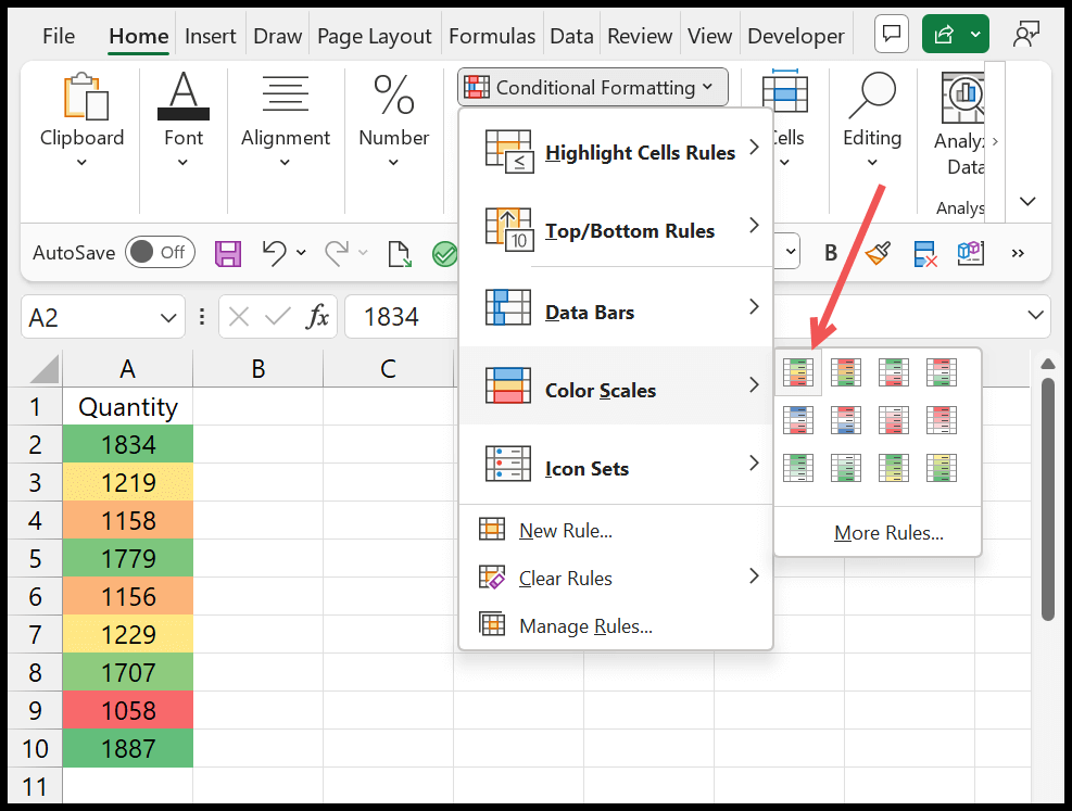
There are 12 pre-defined color scales that you can use here. Each of these color scales is unique. And the color scale we have applied has three colors: green, yellow, and red, which means green for higher values, yellow for mid-range values, and red for lower values.
Note: If you want to hide the numbers from the color scales, open the Format Cells options (Ctrl + 1), click Custom, enter ;;; (three semicolons) in the Type box, and then click OK. The colors stay, and the numbers are hidden.
Create a Custom Color Scale
Apart from the pre-defined scales, you can create a custom rule to apply the color scale to a range of cells. For this, you need to click on “More Rules” in the Color Scales options.

When you click on it, it will show you a new dialog box where you can create a custom color scale.

You can choose “Format Style” from this dialog box to apply a 2-Color Scale or 3-Color Scale.

Once you select the scale you want to apply, you have five ways to create a rule:
1. Lowest/Highest Value
It is the default way to create a rule, and pre-defined rules are based on this. It takes the lowest and the highest value from the range you have selected and creates a rule based on that.
2. Percentage
With percentage, you can specify the percentage for lower, mid, and higher values (3-Scale), or lower and higher (2-Scale). For example, if you specify 10% as the lowest percentage, it will apply the full lower color to the values in the lowest 10% of the range between the smallest and the largest value. And if you use 80% as the highest percentage, it will apply the full higher color to the values in the top 20% of that range. Percent is based on the values, not on how many cells there are.

3. Percentile
Percentile works differently to apply color scales. In the example below, we have used 80 for the highest value, which means all the values at or above the 80th percentile (the top 20% of the values by rank). It will create a group of top values, and the exact same color shade will be applied to all those cells.

Same with the lowest percentile: with 10, all the values at or below the 10th percentile form one group. All the values in this group of values will get the exact color you specified in the minimum color.
Quick Links to Learn More – Link
4. Number
With the number, you can define a custom number by entering it. This option is great to use when using numbers as per a standard. Let’s say you want to apply color based on 0 and 100 as minimum and maximum values.

5. Formula
Sometimes, you might need to get the value by using a formula. Let’s say you want to apply the color scale to a column but want to get the minimum, midpoint, and maximum values from a different column.
In that case, select Formula as the Type for each point and enter formulas like these (here, the other column is C2:C13):
=MIN($C$2:$C$13)
=PERCENTILE($C$2:$C$13,0.5)
=MAX($C$2:$C$13)
Use absolute references (with $), and note that the formula must return a number.

Creating a Color Scale with More than 3 Colors
We don’t have the option to create a 4-color scale or more; in this case, you can create one conditional formatting rule for each color. Below we have a 5-color scale where we have used five different rules.

Each of these five rules uses a different condition.

These five formulas calculate five different slabs of numbers from the range.
- Below 2000
- From 2000 to 3999
- From 4000 to 5999
- From 6000 to 7999
- Above 8000
And for each formula, there is a defined color to apply.
For example, the rule for the second slab (2000 to 3999) uses a formula like the following, written for a range that starts at cell A2:
=AND(A2>=2000,A2<4000)
To create a rule like this, select the range, go to Home ➜ Conditional Formatting ➜ New Rule ➜ Use a formula to determine which cells to format, enter the formula, pick a fill color and click OK. Repeat it for each slab with its own color.
Reverse the Colors of a Color Scale
Sometimes, a lower value is better, like for expenses or delivery days. In that case, you want green for the lowest values and red for the highest. You can pick the Red – Yellow – Green scale from the pre-defined list, or go to Conditional Formatting ➜ Manage Rules, edit the rule, and swap the colors of the Minimum and Maximum.
Things to Know About Color Scales
- Text and blank cells: color scales only color cells with numbers (including dates and times). Text and empty cells stay without a color.
- Error values: if the range has an error like #N/A, the color scale isn’t applied at all, so fix the errors first (for example, with IFERROR).
- Remove a color scale: select the range and go to Home ➜ Conditional Formatting ➜ Clear Rules ➜ Clear Rules from Selected Cells.
- Color-blind readers: red and green are hard to tell apart for many people, so a scale like White – Blue or a 2-color scale is easier to read.
Frequently Asked Questions
What is the difference between Percent and Percentile in a color scale?
Percent is based on the values: 80% means the point that is 80% of the way from the smallest to the largest value. Percentile is based on the rank: the 80th percentile is the value that 80% of the values are below.
Can I apply a color scale based on another column?
Not directly. A color scale colors each cell by its own value. You can only take the minimum, midpoint and maximum from another column with the Formula type. To color cells by another column’s values, use rules with formulas instead, like in the 5-color example above.
Why is my color scale not showing?
The usual reasons are numbers stored as text, an error value in the range, or another rule with a higher priority that colors the same cells. Check the rules in Conditional Formatting ➜ Manage Rules.

Written by
Puneet Gogia
Microsoft MVP — Excel · Founder, Excel Champs
Twelve years of teaching Excel, and a decade before that using it as a data analyst. Every tutorial here is written from a file I actually built.