How to Insert a Check Mark Symbol [Tickmark] in Excel

Last week while traveling I met a person who asked me a smart question. He was quietly working on his laptop and suddenly asked me this:

“Hey, do you know how to insert a check mark symbol in Excel?“

And then I figured out that he had a list of customers and he wanted to add a checkmark for every customer to whom he met.

Well, I showed him a simple way and he was happy with that. But eventually today morning, I thought maybe there is more than one way to insert a checkmark in a cell.

And luckily, I found that there several for this. So today in this post, I’d like to show you how to add a check mark symbol in Excel using 10 different methods and all those situations where we need to use these methods.

Apart from these 10 methods, I have also mentioned how you can format a checkmark + count checkmarks from a cell of the range.

Quick Notes

• In Excel, a checkmark is a character of wingding font. So, whenever you insert it in a cell that cell needs to have a wingding font style (Except, if you copy it from anywhere else).
• These methods can be used in all the Excel versions (2007, 2010, 2013, 2016, 2019, and Office 365).

download this sample file

When You should be using a Check Mark in Excel

A checkmark or tick is a mark that can be used to indicate the “YES”, to mention “Done” or “Complete”.

So, if you are using a to-do list, want to mark something is done, complete, or checked then the best way to use a checkmark.

1. Keyboard Shortcut to Add a Checkmark

Nothing is faster than a keyboard shortcut, and to add a checkmark symbol all you need a keyboard shortcut.

The only thing you need to take care of; The cell where you want to add the symbol must have wingding as font style. And below is the simple shortcut you can use insert a checkmark in a cell.

1. If you are using Windows, then: Select the cell where you want to add it.
2. Use Alt + 0 2 5 2 (make sure to hold the Alt key and then type “0252” with your numeric keypad).
   
3. And, if you are using a Mac: Just select the cell where you want to add it.
4. Use Option Key + 0 2 5 2 (make sure to hold the key and then type “0252” with your numeric keypad).
   

2. Copy Paste a Checkmark Symbol in a Cell

If you usually don’t use a checkmark then you can copy-paste it from somewhere and insert it in a cell

Because you are not using any formula, shortcut, or VBA here (copy paste a checkmark from here ✓).

Or you can also copy it by searching it on google. The best thing about the copy-paste method is there is no need to change the font style.

3. Insert a Check Mark Directly from Symbols Options

There are a lot of symbols in Excel which you can insert from the Symbols option, and the checkmark is one of them.

From Symbols, inserting a symbol in a cell is a brainer, you just need to follow the below steps:

1. First, you need to select the cell where you want to add it.
2. After that, go to Insert Tab ➜ Symbols ➜ Symbol.
   
3. Once you click on the symbol button, you will get a window.
4. Now from this window, select “Winding” from the font dropdown.
5. And in the character code box, enter “252”.
6. By doing this, it will instantly select the checkmark symbol and you don’t need to locate it.
   
7. In the end, click on “Insert” and close the window.

As this is a “Winding” font, and the moment you insert it in a cell Excel changes the cell font style to “Winding”.

Apart from a simple tick mark, there is also a boxed checkmark is there (254) which you can use.

If you want to insert a tick mark symbol in a cell where you already have text, then you need to edit that cell (use F2).

The above method is a bit long, but you don’t have to use any formula or a shortcut key and once you add it into a cell you can copy-paste it.

4. Create an AUTOCORRECT to Convent it to a Check Mark

After the keyboard shortcut, the fast way is to add a checkmark/tick mark symbol in the cell, it’s by creating AUTOCORRECT.

In Excel, there is an option that corrects misspelled words. So, when you insert “clear” it converts it into “Clear” and that’s the right word.

Now thing is, it gives you the option to create an AUTOCORRECT for a word and you define a word for which you want Excel to convert it into a checkmark.

Below are the steps you need to use:

1. First, go to the File Tab and open the Excel options.
   
2. After that, navigate to “Proofing” and open the AutoCorrect Option.
   
3. Now in this dialog box, in the “Replace” box, enter the word you want to type for which Excel will return a checkmark symbol (here I’m using CMRK).
4. Then, in the “With:” enter the checkmark which you can copy from here.
   
5. In the end, click OK.

From now, every time when you enter CHMRK Excel will convert it into an actual check mark.

There are a few things you need to take care which you this auto corrected check mark.

• When you create an auto-correct you need to remember that it’s case-sensitive. So, the best way can be to create two different auto corrects using the same word.
• The word you have specified to be corrected as a checkmark will only get converted if you enter it as a separate word. Let’s say if you enter Task1CHMRK it will not get converted as Task1. So, the text must be Task1 CHMRK.
• The AUTO correct option applied to all the Office Apps. So, when you create a autocorrect for a checkmark you can use it in other apps as well.

5. Macro to Insert a Checkmark in a Cell

If you want to save your efforts and time, then you can use a VBA code to insert a checkmark. Here is the code:

Sub addCheckMark()

Dim rng As Range

For Each rng In Selection
With rng
.Font.Name = "Wingdings"
.Value = "ü"
End With
Next rng

End Sub

Pro Tip: To use this code in all the files you add it into your Personal Macro Workbook.

Here’s how this code works.

When you select a cell or a range of cell and run this code it loops through each of the cells and changes its font style to “Wingdings” and enter the value “ü” in it.

Top 100 Macro Codes for Beginners

Add Macro Code to QAT

This is a PRO tip that you can use if you are likely to use this code more often in your work. Follow these simple steps for this:

1. First, click on the down arrow on the “Quick Access Toolbar” and open the “More Commands”.
2. Now, from the “Choose Commands From” select “Macros” and click on “Add>>” to add this macro code to the QAT.
3. In the end, click OK.

Double-Click Method using VBA

Let’s say you have a to-do list where you want to insert a checkmark just by double-clicking on the cell.

Well, you can make this happen by using VBA’s double-click event. Here I’m using the same code below code:

Private Sub Worksheet_BeforeDoubleClick(ByVal Target As Range, Cancel As Boolean)
If Target.Column = 2 Then
Cancel = True
Target.Font.Name = "Wingdings"
If Target.Value = "" Then
Target.Value = "ü"
Else
Target.Value = ""
End If
End If
End Sub

How to use this code

1. First, you need to open the VBA code window of the worksheet and for this right-click on the worksheet tab and select the view code.
   
2. After that, paste this code there and close the VB editor.
3. Now, come back to the worksheet and double click on any cell in column B to insert a checkmark.

How this code works

When you double-click on any cell this code triggers and checks if the cell on which you have double-clicked is in column 2 or not.

And, if that cell is from column 2 change its font style to “Winding” After that it checks if that cell is blank or not, if the cell is blank then enter the value “ü” in it which converts into a checkmark as it has already applied the font style to the cell.

And if a cell has a checkmark already then you remove it by double-clicking.

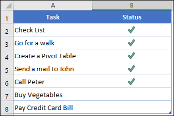
6. Add a Green Check Mark with Conditional Formatting

If you want to be more awesome and creative, you can use conditional formatting for a checkmark.

Let’s say, below is the list of the tasks you have where you have a task in one column and a second where you want to insert a tick mark if the task is completed.

Below are the steps you need to follow:

• First, select the target cell or range of cells where you want to apply the conditional formatting.
• After that go to Home Tab ➜ Styles ➜ Conditional Formatting ➜ Icon Sets ➜ More Rules.
• Now in the rule window, do the following things:
  
• Select the green checkmark style from the icon set.
• Tick mark the “Show icon only” option.
• Enter “1” as a value for the green checkmark and select a number from the type.
• In the end, click OK.

Once you do that, enter 1 in the cell where you need to enter a checkmark, and because of conditional formatting, you will get a green checkmark there without the actual cell value.

If you want to apply this formatting from one cell or range to another range you can do it by using format painter.

7. Create a Dropdown to Insert a Checkmark

If you don’t want to copy-paste the checkmark and don’t even want to add the formula, then the better way can be to create a drop-down list using data validation and insert a checkmark using that drop-down.

Before you start make sure to copy a checkmark ✓ symbol before you start and then select the cell where you want to create this dropdown. And after that follow these simple steps to create a drop-down for adding a checkmark:

• First, go to Data tab ➨ Data Tools ➨ Data Validation ➨ Data Validation.
  
• Now from the dialog box, select the “List” in the drop down.
• After that, paste the copied check mark in the “Source”.
  
• In the end, click OK.
  

If you want to add a cross symbol ✖ along with the tick mark so that you can use any of them when you need simply add a cross symbol using a comma and click OK.

There’s one more benefit that drops down gives that you can disallow any other value in the cell other than a checkmark and a cross mark.

All you need to do is go to the “Error Alert” tab and tick mark “Show error alert after invalid data is entered” after that select the type, title, and message to show when a different value is entered.

Related

• How to Create a Dependent Dropdown List in Excel
• How to Create a Dynamic Dropdown List in Excel

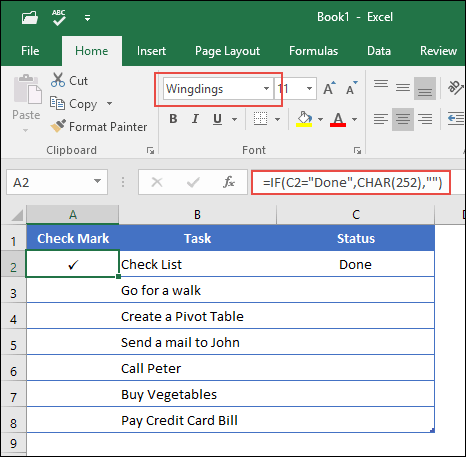
8. Use CHAR Function

Not all the time you need to enter a checkmark by yourself. You can automate it by using a formula as well. Let’s say you want to insert a checkmark based on a value in another cell.

Like below where when you enter value done in column C the formula will return a tick mark in column A. To create a formula like this we need to use CHAR function.

CHAR(number)

Related: Excel’s Formula Bar

Quick INTRO: CHAR Function

CHAR function returns the character based on the ASCII value and Macintosh character set.

Syntax:

CHAR(number)

…how does it work

As I say CHAR is a function to convert a number into an ANSI character (Windows) and Macintosh character set (Mac). So, when you enter 252 which is the ANSI code for a checkmark, the formula returns a checkmark.

9. Graphical Checkmark

If you are using OFFICE 365 like me, you can see there is a new tab with the name “Draw” there on your ribbon.

Now the thing is: In this tab, you have the option to draw directly into your spreadsheet. There are different pens and markers which you can use.

And you can simply draw a simple checkmark and Excel will insert it as a graphic.

The best thing is when you share it with others, even if they are using a different version of Excel, it shows as a graphic. There’s also a button to erase as well. You must go ahead and explore this “Draw” tab there are a lot of cool things which you can do with it.

10. Use Checkbox as a Checkmark in a Cell

You can also use a checkbox as a checkmark. But there is a slight difference between both:

1. A checkbox is an object which is like a layer which placed above the worksheet, but a checkmark is a symbol which you can insert inside a cell.
2. A checkbox is a sperate object and if you delete content from a cell checkbox won’t be deleted with it. On the other hand, a checkmark is a symbol which you inside a cell.

Here’s the detailed guide which can help you to learn more about a checkbox and using it in a right way.

11. Insert a Checkmark (Online)

If you use Excel’s online App then you need to follow a different way to put a checkmark in a cell.

The thing is, you can use the shortcut key but there is no “Winding” font there, so you can’t convert it into a checkmark. Even if you use the CHAR function it won’t be converted into a checkmark.

But…But…But…

I’ve found a simple way by installing an app into Online Excel for symbols to insert check marks. Below are the steps you need to follow:

• First, go to the Insert Tab ➜ Add-Ins and then click on the office Add-Ins.
  
• Now, in the add-ins window, click on the store and search for the “Symbol”.
• Here you’ll have an add-in with the name of “Symbol and Characters”, click on the add button to install it.
  
• After that, go to the Add-Ins tab and open the add-in which you have just installed.
• At this point, you have a side pane where you can search for the checkmark symbol and double click on it to insert it into the cell.
  

Yes, that’s it.

…make sure to get this sample file from here to follow along and try it yourself

Some of the IMPORTANT Points YOU need to learn

Here are a few points which you need to learn about using checkmarks.

1. Formatting a Checkmark

Formatting a check mark can be required sometimes especially when you are working with data where you are validating something. Below are the things which you can do with a checkmark:

• Make it bold and italic.
• Change its color.
• Increase and decrease font size.
• Apply an underline.

2. Deleting a Checkmark

Deleting a check mark is simple and all you need to do is select the cell where you have it and press the delete key.

Or, if you have text along with a checkmark in a cell then you can use any of the below methods.

1. First, edit the cell (F2) and delete the checkmark.
2. Second, replace the checkmark with no character using find and replace option.

3. Count Checkmarks

Let’s say want to count the checkmark symbols you have in a range of cells. Well, you need to use formula by combining COUNTIF and CHAR and the formula will be:

=COUNTIF(G3:G9,CHAR(252))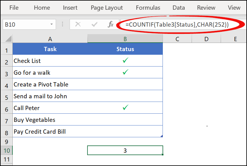

In this formula, I have used COUNTIF to count the characters which are returned by the CHAR.

…make sure to check this sample file from here to follow along and try it yourself

In the end,

A check mark is helpful when you are managing lists.

And creating a list with checkmarks in Excel is no big deal now, as you know more than 10 methods for this. From all the methods above, I always love to use conditional formatting……and sometimes copy-paste.

You can use any of these which you think is perfect for you. I hope this tip will help you in your daily work. But now tell me one thing.

Have you ever used any of the above methods? Which method is your favorite?

Make sure to share your views with me in the comment section, I’d love to hear from you. And please, don’t forget to share this post with your friends, I am sure they will appreciate it.