Combining values with CONCATENATE is the best way, but with this function, it’s not possible to refer to an entire range. You need to select all the cells of a range one by one, and if you try to refer to an entire range, it will return the text from the first cell.
In this situation, you do need a method where you can refer to an entire range of cells to combine them in a single cell. Today in this post, I’d like to share with you 5 different ways to combine text from a range into a single cell.
[CONCATENATE + TRANSPOSE] to Combine Values
The best way to combine text from different cells into one cell is by using the transpose function with concatenating function.
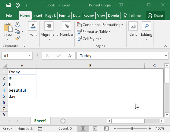
Look at the below range of cells where you have a text, but every word is in a different cell and you want to get it all in one cell. Below are the steps you need to follow to combine values from this range of cells into one cell.
- In the B8 (edit the cell using F2), insert the following formula, and do not press enter.
- =CONCATENATE(TRANSPOSE(A1:A5)&” “)
- Now, select the entire inside portion of the concatenate function and press F9. It will convert it into an array.
- After that, remove the curly brackets from the start and the end of the array.
- In the end, hit enter.

That’s all.
How this formula works
In this formula, you have used TRANSPOSE and space in the CONCATENATE. When you convert that reference into hard values it returns an array. In this array, you have the text from each cell and a space between them and when you hit enter, it combines all of them.
Combine Text using the Fill Justify Option
Fill justify is one of the unused but most powerful tools in Excel. And, whenever you need to combine text from different cells you can use it. The best thing is, that you need a single click to merge text. Have look at the below data and follow the steps.
- First of all, make sure to increase the width of the column where you have text.
- After that, select all the cells.
- In the end, go to Home Tab ➜ Editing ➜ Fill ➜ Justify.
This will merge text from all the cells into the first cell of the selection.
TEXTJOIN Function for CONCATENATE Values
If you are using Excel 2016 (Office 365), there is a function called “TextJoin”. It can make it easy for you to combine text from different cells into a single cell.
Syntax:
TEXTJOIN(delimiter, ignore_empty, text1, [text2], …)
- delimiter a text string to use as a delimiter.
- ignore_empty true to ignore blank cell, false to not.
- text1 text to combine.
- [text2] text to combine optional.
how to use it
To combine the below list of values you can use the formula:
=TEXTJOIN(" ",TRUE,A1:A5)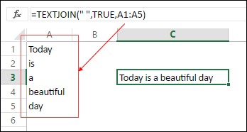
Here you have used space as a delimiter, TRUE to ignore blank cells and the entire range in a single argument. In the end, hit enter and you’ll get all the text in a single cell.
Combine Text with Power Query
Power Query is a fantastic tool and I love it. Make sure to check out this (Excel Power Query Tutorial). You can also use it to combine text from a list in a single cell. Below are the steps.
- Select the range of cells and click on “From table” in data tab.

- If will edit your data into Power Query editor.

- Now from here, select the column and go to “Transform Tab”.
- From “Transform” tab, go to Table and click on “Transpose”.

- For this, select all the columns (select first column, press and hold shift key, click on the last column) and press right click and then select “Merge”.

- After that, from Merge window, select space as a separator and name the column.

- In the end, click OK and click on “Close and Load”.
Now you have a new worksheet in your workbook with all the text in a single cell. The best thing about using Power Query is you don’t need to do this setup again and again.
When you update the old list with a new value you need to refresh your query and it will add that new value to the cell.
VBA Code to Combine Values
If you want to use a macro code to combine text from different cells then I have something for you. With this code, you can combine text in no time. All you need to do is, select the range of cells where you have the text and run this code.
 Sub combineText()
 Dim rng As Range
 Dim i As String
 For Each rng In Selection
 i = i & rng & " "
 Next rng
 Range("B1").Value = Trim(i)
 End Sub
Make sure to specify your desired location in the code where you want to combine the text.
In the end,
There may be different situations for you where you need to concatenate a range of cells into a single cell. And that’s why we have these different methods.
All methods are easy and quick, you need to select the right method as per your need. I must say that give a try to all the methods once and tell me:
Which one is your favorite and worked for you?
Please share your views with me in the comment section. I’d love to hear from you, and please, don’t forget to share this post with your friends, I am sure they will appreciate it.
I have a list of different tags i need to put together in a different sheet for convenience, problem is that values pulled from other documents does not increase when copied to new cell, how to i make the numbers after the $ to increase with 1? (In the string below id like $58 and $69 to increase when i copy to new cell by dragging downwards)
=CONCATENATE(‘[PLCTagsASi.xlsx]PLC Tags’!$A$58;”_”;'[PLCTagsASi.xlsx]PLC Tags’!$D$60)
Hi the VBA portion works almost exactly for what I need. I changed the separator though to be ” || “. Doing this of course yields combined numbers separated by a space, two || symbols, and another space. However, they come out as 0943 || 0957 || 0960 || 0963 || and as you can see it puts those || symbols at the end. Is there a way to not have it put the space and the two || symbols after the last number? So that when it combines them it would only be 0943 || 0957 || 0963? If the macro can do that, that would be exactly what I need it for. Would that be an edit to the VBA and what would that edit be? Please and thank you so much!
#1 is of no use, string value is fixed at moment when concat & transpose formula written.
Super helpful post RE concatenation of a range of cells in XLS; thank you!
All your solutions are excellent.
Many different methods are also taught.
Though I am very good at Excel, I learn many many things from your website.
THANKS A LOT.
God Bless.
Great help!
115750-760 ,765how to convert in column with serial wise
Hi,
You’re a genius. Very very help for me. Thanks a lot.
Regards,
Al-Amin
Hello,
Is it possible via formula, w/o vba nor Power Tools, to combine 2 arrays (generated by formula) into a non-array value separated by comas. Textjoin will work with only 1 array but returns the first element when there is a division of array inside the Textjoin formula. I also tried to have another cell to do the division w/o luck. If u need to know why I’m doing this, I’ll be glad to add more details.
TQ, KR!
Thank you so much for this, the formula worked perfectly – saved me ages. Thanks 🙂
😉
Thank you for this VBA code. It works great! However, I want to add one more aspect to the code and I can’t quite figure it out.
I would like for the code to locate a cell, based on a certain text, then select everything in the list below that cell. Is that something easily doable?
Good morning.
Thanks for the interesting article. Unfortunately, as far as I can see, none of the methods actually does what I want.
I am writing an accounting spreadsheet, and I want a column that shows an error message if there is anything unexpected in the columns where I enter data, or in the calculation columns. At present, it is a huge long tangle of nested if statements and messages joined by “&” operators. I want to simplify this by setting up some columns, each of which detects a particular error, and generates an appropriate message if it finds it. This will make it much easier to add more error checking in future – just insert more columns in this part of the sheet.
In this scenario, the error message column (the one that is always visible) needs to be a concatenation of all the individual error columns.
The first two methods don’t work, since they use the values of the cells at the time you type the formula, while I want one that continually updates as the data – and messages – change.
The third method doesn’t work because I am using the standalone Excel 2016, which doesn’t have TEXTJOIN. This is particularly frustrating, because TEXTJOIN is exactly the function I need!
One day, I intend to add some VBA code to my spreadsheet to cover things like year end (when I have to chop off a year’s worth of data and replace it with a few lines of carried-forward values), but I have never programmed in VB (of any flavour), so this is going to be a major project. (Maybe I’ll use Python code instead.) The problem I foresee here is that code generally executes when the user clicks a button; formulae execute when you change a cell on which they depend. If I set up a VBA program to execute every time I enter data, and it computes this for every line of the spreadsheet, it introduces a huge processing overhead! And if I (or anyone else using the sheet) can remember to click a “check for errors” button, we can remember to check for errors anyway.
So this leaves Power Query. I’d never even heard of this tool before I read your article! If (as I suspect) I need to click something to refresh my query in order to check for errors, then it suffers from the same problem as VBA. But it’s worth further investigation. Thank you for bringing it to my attention.
Maybe I need to migrate to Excel 2019. Now that I have (I think) sorted out all the bugs that were introduced when I migrated from Excel 2007 to Excel 2016, that’s a possibility. (The bugs mostly concerned the changed behaviour of SUMIF when the data range and criterion range were different lengths)
In the meantime, I shall probably set up the columns I need, and concatenate them with & or CONCATENATE. I’ll just have to remember to add more arguments to the formula whenever I add more error checking columns.
Philip.
Philip
This may be a bit out of date now. However, if the above VBA is adjusted, it can be used to return the concatenated strings as a normal formula, enter (something like) the following into a VBA module (Alt-F11, Insert-Module):
“Public Function RANGECAT(rng1 As Range, Optional rng2 As Range) As String
Dim r1 As Integer, c1 As Integer, r2 As Integer, c2 As Integer
Dim cel As String
cel = “”
For c1 = 1 To rng1.Columns.Count
For r1 = 1 To rng1.Rows.Count
cel = cel + rng1.Cells(r1, c1)
Next r1
Next c1
If rng2 Is Nothing Then
Else
For c2 = 1 To rng2.Columns.Count
For r2 = 1 To rng2.Rows.Count
cel = cel + rng2.Cells(r2, c2)
Next r2
Next c2
End If
RANGECAT = cel
End Function”
The “combineText = cel” returns the value found. Further ranges can be added as needed (using “Optional rng3 as range, …” and repeating the rng2 for loops).
Hope it helps
Hi Puneet,
I have 1 Query in VBA Example : Ship Mode : Instant Air
And Customer Name’s : Jeremy Lonsdale
Cindy Schnelling
Susan Vittorini
Toby Braunhardt
Ralph Arnett
Harold Engle
Helen Abelman
Guy Armstrong
Jennifer Braxton
Giulietta Baptist
And I need the result is Instant Air
Roy Skaria, Jeremy Lonsdale, Cindy Schnelling, Susan Vittorini, Toby Braunhardt, Ralph Arnett, Harold Engle, Helen Abelman, Guy Armstrong, Jennifer Braxton, Giulietta Baptist, Erica Bern, Christopher Schild, Joy Smith, Evan Minnotte, Jenna Caffey,
Like this Instant Air Would be one line remaining all are in one line with commas how it is possible can you let me know.