Excel 3D Reference (A Simple and Quick Guide to Understand)

We all want to save time. And, using 3D Reference in Excel can save a lot of time.

It is like a three-dimensional chart or image with more than one phase. A normal range is all about a group of cells from a single worksheet.

For Example, in =SUM(Sheet1!A1:A10), “A1:A10” is a group of cells that is referred from Sheet1.

But, a 3D reference is a range of cells in which you can refer to the same cells from multiple worksheets using a single reference.

In simple words, refer to the same cell or range from multiple sheets.

Create a 3D Reference

The only thing which you have to take care of before using a 3D reference is all the worksheets should be in a sequence. Let me show you an example.

Now here you have 5 worksheets in a workbook. So, if you want to calculate a sum of the range C5:D6 from all 5 worksheets you have to use a formula like the one below.

=('2009'!A1:A10,'2010'!A1:A10,'2011'!A1:A10,'2012'!A1:A10,'2013'!A1:A10)

But if you want to create a 3D formula with a 3D reference, it will look something like this.

=SUM('2009:2013'!A1:A10)

How 3D Reference Works in Excel

A 3D range formula always works in two different parts.

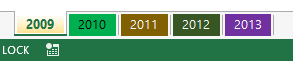
• First – a range of worksheets: Like a range of cells, you have to create a range of worksheets from which you want to refer cells. The range of worksheets must be continuous. In the above example, I have five worksheets from 2009 to 2013.
• Second – A range of cells. This is a normal range of cells that you want to refer to in all the worksheets.

Adding a New Worksheet

If you add a new worksheet within the span of sheets referenced by a 3D formula, Excel will automatically include that sheet in the 3D reference.

Suppose you insert a worksheet between 2009 to 2013.

It will automatically include the value of the range A1:A10 from the new sheet in the function you are using.

Deleting a Worksheet

If you delete a worksheet from 2009 to 2013. It will automatically exclude the value of cell C4 from the function you are using.

Moving a Sheet

Moving a worksheet to a position outside of the referenced span of sheets will no longer be included in the calculation.

In this example, the range of worksheets starts from “Sheet 2009” and ends at “Sheet 2013.”

The point is that if you move any sheet out of this range, that sheet will be excluded from the formula calculation.

Functions which Supports 3D-Reference

• SUM: Used to add up the same cell or range of cells across multiple worksheets.
• AVERAGE: Calculates the average of the same cell or range of cells over multiple worksheets.
• MAX: Determines the highest value in the same cell or range of cells over multiple worksheets.
• MIN: Identifies the lowest value in the same cell or range of cells over multiple worksheets.
• COUNT: This function counts the number of cells with numerical data in the same cell or range of cells across multiple worksheets.
• PRODUCT: Multiplies all the numbers given in a set of cells.
• COUNTA: Counts the number of cells that are not empty in a range.
• STDEV.P: Calculates the standard deviation based on the entire population given as arguments.
• VARP: Calculates variance based on the entire population.

Conclusion

One of the most important benefits of 3D references is that they can shorten complex formulas.

You don’t have to refer to all the worksheets separately in formulas. And I hope this method will help you write better formulas.

Now tell me one thing. Have you tried it before? Please share your views with me in the comment section.

I’d love to hear from you. And please don’t forget to share with your friends.