

To turn “John Smith” into “Smith, John”, the trick is to join the name to itself and then take a slice from the middle: =MID(A1&", "&A1,SEARCH(" ",A1)+1,LEN(A1)+1). Doubling the text means the last name and the first name end up next to each other across the join, so a single MID starting just after the space picks up both in the right order.
In Excel 365 there’s a far more readable version: =TEXTAFTER(A1," ")&", "&TEXTBEFORE(A1," "). The classic two-part version works in any release: =MID(A1,SEARCH(" ",A1)+1,LEN(A1))&", "&LEFT(A1,SEARCH(" ",A1)-1).
Two limits to know. A cell holding a single word returns #VALUE!, because SEARCH can’t find a space — wrap it in =IFERROR(...,A1) to leave those unchanged.
And a middle name goes to the wrong side: “John Paul Smith” becomes “Paul Smith, John”, since the formula splits at the first space. For a one-off conversion with no formula, type the flipped version next to the first row and press Ctrl+E for Flash Fill.
To flip the names (First and Last) into last and first names in Excel, you need to use a combination of MID, LEN, and SEARCH functions. In this tutorial, we will learn to write a formula for this.

Excel Formula to Swap First and Last Names
You can use the following steps to write this formula:
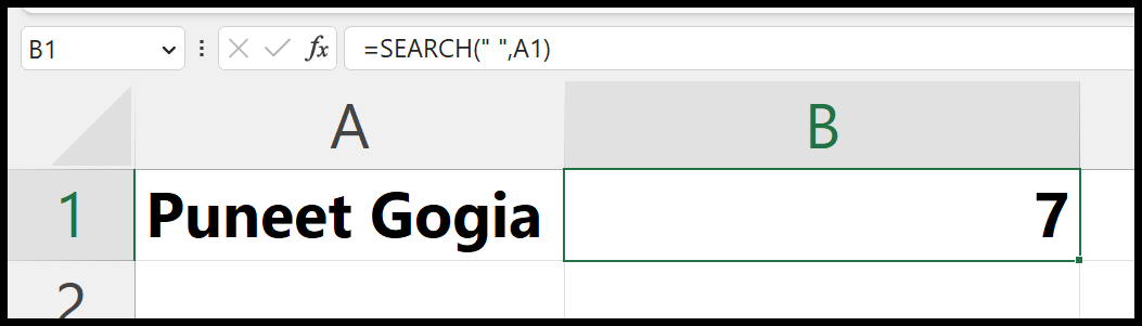
- First, you need to use the SEARCH function to find the space that you have between both first and last names.
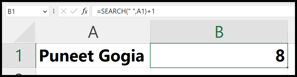
- After that, add one to the number returned by the SEARCH.
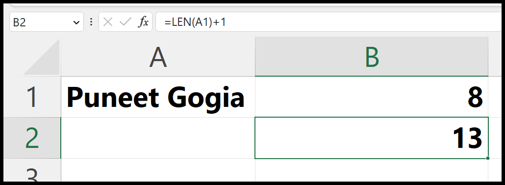
- Next, you need to use the LEN function to get the count of total characters (first and last name). And add 1 into it also.
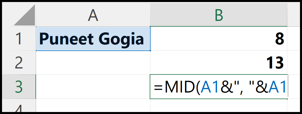
- Now, enter the MID function, and in the first argument, enter the A1 cell (where you have the name) twice by combining it with a comma and space.
- From here, in the second and third arguments of the MID, enter the SEARCH function and LEN function (which we have written in the earlier steps) respectively.
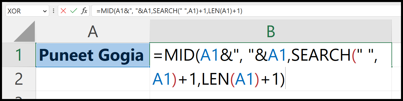
- In the end, hit enter to get the result.
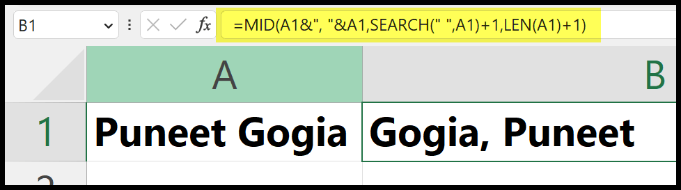
=MID(A1&", "&A1,SEARCH(" ",A1)+1,LEN(A1)+1)How Does This Formula Works
To understand this formula, you need to split it into three parts. The main function is the MID function and we have three arguments in the mid function to define, and that’s why you need to split this formula into three parts to understand it.

In the FIRST PART, we have the text argument of the MID. And in this argument, we have combined the first and the last names twice using a comma and a space.

In the SECOND PART, you have the SEARCH function that refers to cell A1 where you have the names (first and last) and look for the space in it, and then add 1 in it. This way you get the starting position of the last name from the cell.

In the THIRD PART, you have the LEN function that counts the total number of characters from the original names (first and last) and adds 1 to it.
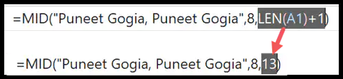
In the end, the MID function gets the last name from the first value, and the first name from the second value to give you the result of swapping the first name and the last name into the last and first name.
Written by
Puneet Gogia
Microsoft MVP — Excel · Founder, Excel Champs
Twelve years of teaching Excel, and a decade before that using it as a data analyst. Every tutorial here is written from a file I actually built.