Count Days Between Two Dates (COUNTIF Date Range) in Excel

To count days between two dates (a range of dates), you need to use the COUNTIFS function instead of COUNTIF. To create a date range, you need to specify a lower date and an upper date. This tells Excel to count only days between the range of days.

Formula to Count Days Between Two Dates

You can use the following steps:

1. First, enter the COUNTIFS function in a cell.
2. After that, in the criteria_range1 argument, refer to the range where you have dates.
3. Next, in the criterai1 argument, enter the greater than (>) and equal sign (=) and enclose between double quotation marks. And then, refer to the cell where you have the lower date.
4. Now, in the criteria_range2, refer to the date range again.
5. After that, in criteria2, enter the lower than (<) and equal sign (=) and enclose it between double quotation marks. And then, refer to the cell where you have the upper date.
6. In the end, close the function and hit enter to get the result.

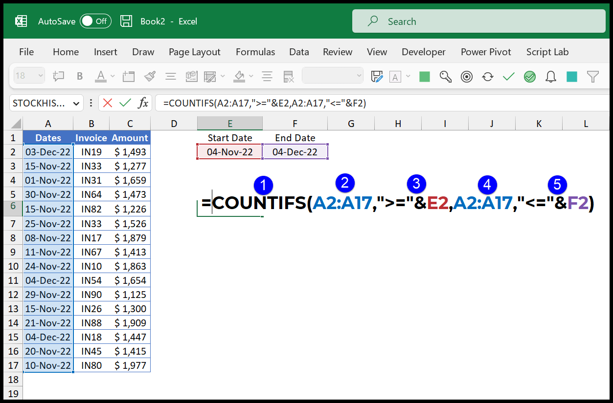
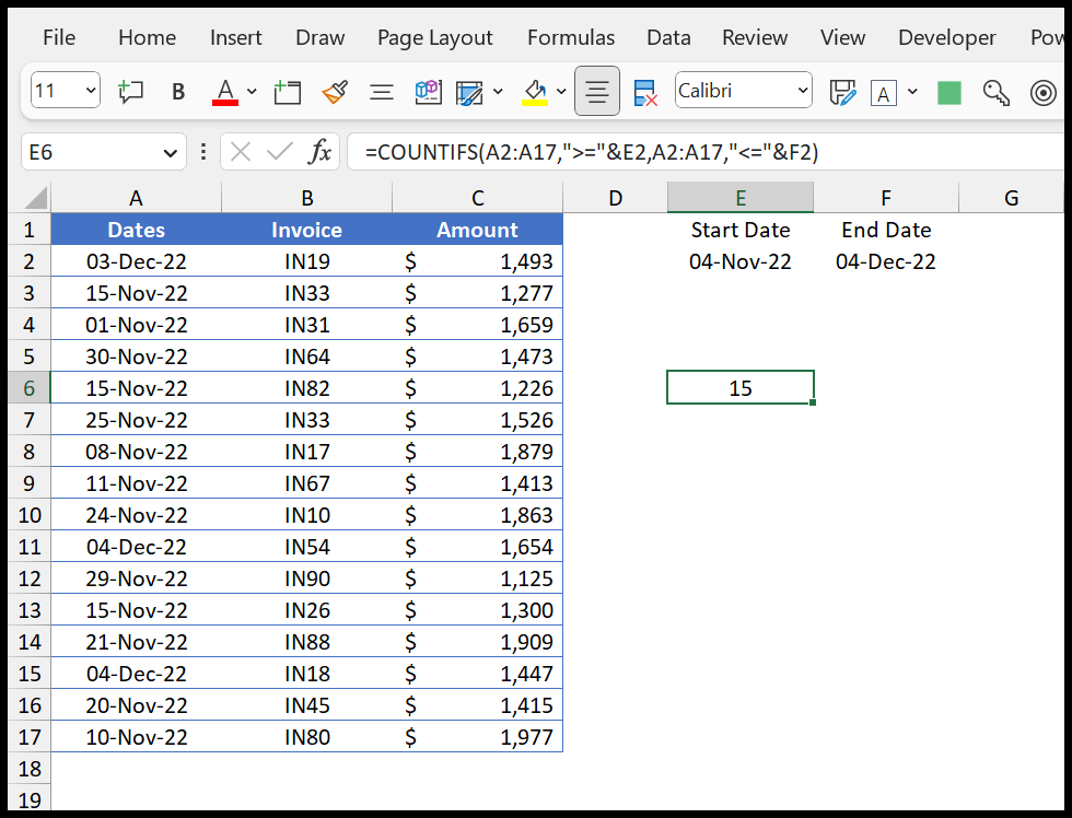
=COUNTIFS(A2:A17,">="&E2,A2:A17,"<="&F2)

How this Formula Works

To understand this formula, you can break it down into two parts.

• In the first part, you have the condition to test for the cells greater than and equal to the date you have in cell E2. i.e., 4-Nov-2022.
• In the second part, you have the condition to test for the cells which are lower than and equal to the date you have in cell F2. i.e., 4-Dec-2022.

So 15 cells have dates between the date range 4-Nov-2022 and 4-Dec-2022.

Note: Make sure to enter greater than (>), lower than (<), and equal (=) operators as text and surrounded by double quotation marks.

Use SUMPRODUCT to Count Between Dates

You can also use SUMPRODUCT to count dates between two dates, just like the following example:

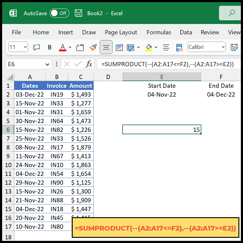
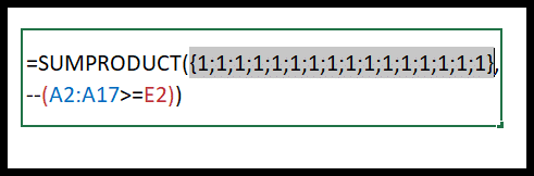
=SUMPRODUCT(--(A2:A17<=F2),--(A2:A17>=E2))

Now let’s understand this formula step by step. But before that, you need to know that SUMPRODUCT can take an array in a single cell.

In the first part of the formula, you have a condition to check all the dates from the range. It will check which is lower and equal to the specified date. You can see it returns TRUE and FALSE.

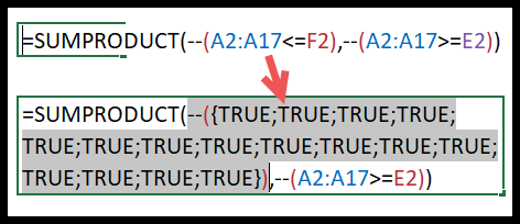
After that, you have a double minus sign that converts these TRUE and FALSE into 1 and 0.

In the second part of the formula, you again have the condition to test. And it returns TRUE if that condition is met, else FALSE.

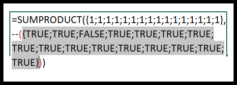
After that, the double minus sign converts TRUE and FALSE into 1 and 0.

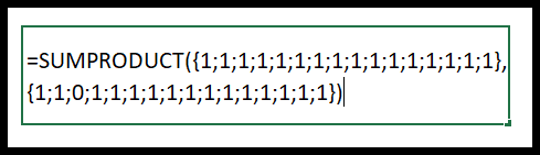
At this point, you have two arrays. 1 means that the date in the range is between the specified date range.

SUMPRODUCT creates a product of these arrays and returns a single array, then sums values from that array which is the count of dates between the range.