Sometimes working with data is not that easy, sometimes we face complex problems.
Let’s say, you want to search for the text “Delhi” from the data. But, in that data, you have the word “New Delhi” not “Delhi”. Now, in this situation, you can’t match or search. Here, you need a way that allows you to use only available value or partial value (Delhi) to match or search for the actual value (New Delhi). Excel Wildcard Characters are meant for this. These wildcard characters are all about searching/looking up a text with a partial match. In Excel, the biggest benefit of these characters is with lookup and text functions. It gives you more flexibility when the value is unknown or partially available.
So today, in this post, I’d like to tell you what wildcard characters are, how to use them, their types, and examples to use them with different functions. Let’s get started.
What is Excel Wildcard Characters
Excel Wildcard Characters are special kinds of characters that represent one or more other characters. It’s used in regular expressions, by replacing them with unknown characters. In simple words, when you are not sure about an exact character to use, you can use a wildcard character in that place.
Types of Excel Wildcard Characters
In Excel, you have 3 different wildcard characters Asterisk, Question Mark, and Tilde. And each of these has its own significance and usage.
Ahead we’ll discuss each of these characters in detail so that you would be able to use them in different situations.
1. Asterisk(*)
An asterisk is one of the most popular wildcard characters. It can find any number of characters (in sequence) from a text. For example, if you use Pi* it will give you words like Pivot, Picture, Picnic, etc.
If you notice, all these words have Pi in starting and then different characters after that. Let’s understand it’s working with an example. Below you have data where you have names of cities and their classification in a single cell.

Now from here, you need to count the number of cities in each classification. and for this, you can use an asterisk with COUNTIF.
=COUNTIF(City,Classification&”*”)
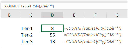
In this formula, you have combined classification text from the cell with an asterisk. So, the formula only matches the classification text in the cell and the asterisk works as the rest of the characters. And in the end, you get the count of cities according to classification.
2. Question Mark
With a question mark, you can replace one single character from a text. In simple words, it helps you get more specific, still using a partial match. For example, if you use c?amps it will return champs and chimps from the data.
3. Tilde (~)
The real use of a tilde is to nullify the effect of a wildcard character. For example, let’s say you want to find the exact phrase pivot*. If you use pivot* as a string, it will give you any word that has champs at the beginning (such as pivot table, or pivot chart).
To specifically the string pivot*, you need to use ~. So, your string would be pivot~*. Here, ~ ensures that Excel reads the following character as is, and not as a wildcard.
Wildcard Characters with Excel Functions
We can easily use all three wildcard characters with all the top functions. Functions like VLOOKUP, HLOOKUP, SUMIF, SUMIFS, COUNTIF, COUNTIFS, SEARCH, FIND, and Reverse LOOKUP.
You can extend this list with all the functions that you use for matching a value, for lookups, or for finding a text. Ahead, I’ll share with you some examples with functions + find and replace options + conditional formatting + with numbers.
1. With SUMIF
Below you have data where you have invoice numbers and their amount. And, we need to sum amounts where invoice numbers have “Product-A” in starting.
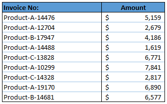
To do this we can use SUMIF with wildcard characters. The formula will be:
=SUMIF(F2:F11,”Product-A*”,G2:G11)

In the above example, we have used an asterisk with the criteria at the end. As we have learned an asterisk can find a partial text with any number of sequence characters.
And, here we have used it with “Product-A”. So, it will match the values where “Product-A” is at the beginning of the value.
2. With VOOKUP
Let’s say you have a list of students with full name and their marks. Now, you want to use VLOOKUP to get marks in another list in which you only have their first names.
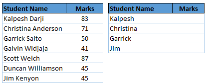
For this, the formula will be:
=VLOOKUP(first_name&”*”,marks_table,2,0)
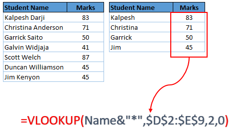
In the above example, you have used vlookup with an asterisk to get marks by only using the first name.
3. For Find and Replace
Using wildcard characters with the find and replace option can do wonders for your data.
In the above example, you have the word “ExcelChamps” which has different characters between it.
And you want to replace those characters with a simple space. You can even do this by using replace option but in that case, you have to replace each character one by one. But you can use a question mark (?) to replace all the other characters with space.
Find “Excel?Champs” & replace it with “Excel Champs” to remove all unwanted characters.
4. In Conditional Formatting
You can also use these wildcard characters with conditional formatting. Let’s say, from a list, you want to highlight the name of the cities which are starting with the letter A.
- First of all, select the first entry from the list and then go to Home → Styles → Conditional Formatting.
- Now, click on the “New Rule” option, and select use a formula to determine which cells to format”.
- In the formula input box, enter =IF(COUNTIF(E2,”A*”),TRUE,FALSE).
- Set the desired formatting, you want to use to highlight.

- Now, I have used conditional formatting in the first cell of the list & I have to apply it to the entire list.
- Select the first cell on which you have applied your formatting rule.
- Go to Home → Clipboard → format painter.
- Select the entire list and it will highlight all the names starting with the letter A.
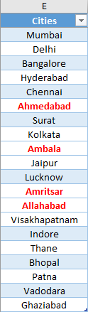
5. Filter values
Wildcard characters work like magic in filters. Let’s say you have a list of cities, and you want to filter city names starting from A, B, C, or any other letter. You can use A* or B* or C* for that.
This will give you the exact name of cities that are starting from that letter. And, if you want to search for any character which is ending with a specific letter you can use it before that letter (*A, *B,*C, etc.).
6. With Numbers
You can use these wildcards with numbers but you have to convert those numbers into text.
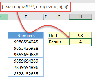
In the above example, you have used the match function and text function to perform a partial match. The text function returns an array by converting the entire range into the text and after that match function, lookup for a value starting from 98.
Sample File
Download this sample file from here to learn more.
Conclusion
With wildcard characters, you can enhance the power of functions when your data is not in a proper format.
These characters help you search or match a value using a partial match which gives you the power to deal with irregular text values. And the best part is you have three different characters to use.
Have you ever used these wildcard characters before?
Share your views with me in the comment section, I’d love to hear from you. And don’t forget to share this tip with your friends.
Related Formulas
-
Back to the List of Excel Formulas