

Excel has no built-in gauge, so you build a speedometer from a doughnut chart for the coloured bands and a pie chart for the needle. Enter your band sizes in one column and add a last value equal to their total, for example 30, 40, 20, 10 and 100, then select it and go to Insert → Insert Pie or Doughnut Chart → Doughnut.
Right-click the ring, choose Format Data Series and set Angle of first slice to 270°. The big last slice drops to the bottom half: give it No Fill and colour the other bands from red to green.
For the needle, use three cells: the value you are tracking on a 0–100 scale in B10, a needle width such as 1 in B11, and =200-B10-B11 in B12. Add them as a second series with Select Data → Add, right-click that series, choose Change Series Chart Type and set it to Pie.
Set the pie’s Angle of first slice to 270° as well and give its first and third slices No Fill. The thin middle slice is your needle; a Point Explosion of about 5% on it makes it stand out from the dial.
To show the reading, insert a text box, click in the formula bar, type =, click B10 and press Enter. The label and the needle now move whenever the value changes.
If the needle points to the wrong place, check that the bands add up to 100 and the three needle cells add up to exactly 200. For any other scale, convert first: with the actual in C2 and the target in D2, put =MIN(100,C2/D2*100) in B10 so the needle never swings past the end of the dial.
When it comes to presenting data in an understandable way in Excel, charts stand out. And there are a few charts which are specific and can be used to present a specific kind of data.
A SPEEDOMETER [Gauge] is one of those charts.
It’s a kind of thing which you can find in your day-to-day life [Just look at the SPEEDOMETER in your car].
And in today’s post, I’m going to show you exactly how to create a SPEEDOMETER in Excel. But here’s the kicker: It’s one of the most controversial charts as well.
So today in this post, we will be exploring it in all the ways so that you can use it in your Excel dashboards when it’s actually required.
What is an Excel SPEEDOMETER Chart?
An Excel SPEEDOMETER Chart is just like a speedometer with a needle which tells you a number by pointing it out on the gauge and that needle moves when there is a change in the data. It’s a single-point chart which helps you to track a single data point against its target.

Steps to Create a SPEEDOMETER in Excel
Here are the steps to create a SPEEDOMETER [Gauge] in Excel which you need to follow.
As I said, we need to insert two doughnut charts and a pie chart but before you start to create a SPEEDOMETER, you need to arrange data for it.
In the below worksheet, we have three different data tables (two for doughnut charts and one for the pie chart). You can DOWNLOAD it from here to follow along.
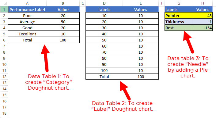
- The first data table is to create the category range for the final SPEEDOMETER which will help you to understand the performance level.
- The second data table is for creating labels ranging from 0 to 100. You can change it if you want to have a different range.
- And in the third data table, we have three values which we will use to create the pie chart for the needle. The pointer value is the real value which you want to track.
To create a SPEEDOMETER in Excel, you can use the below steps:
To create a SPEEDOMETER in Excel, you can use the below steps:
- First of all, go to Insert Tab ➜ Charts ➜ Doughnut Chart (with this you’ll get a blank chart).

- Now, right-click on the chart and then click on “Select Data”.
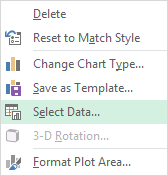
- In the “Select Data” window, click on “Add” under “Legend Entries (Series)” and enter “Category” in the Series name box. After that, select the “Value” column from the first data table.

- Once you click OK, you’ll have a doughnut chart just like below.

- From here, the next thing is to change the angle of the chart, and for this, right-click on the chart and then click on “Format Data Series”.
- In “Format Data Series”, enter 270° in “Angle of first slice” and hit enter.

- After this, you need to hide the bottom half of the chart. For this, click on only that part of the chart and open “Format Data Point” and select “No Fill”.
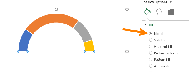
- For the rest of the four data points, I’ve used four different colors (Red, Yellow, Blue, and Green). At this point, you’ll have a chart like below and the next thing is to create the second doughnut chart to add labels.

- Now, right-click on the chart and then click on “Select Data”.
- In the “Select Data Source” window, click on “Add” to enter a new series under “Legend Entries” and select the “Values” column from the second data table.

- Once you click OK, you’ll have a doughnut chart just like below.

- Again, you need to hide the bottom half of the chart by using “No Fill” for color and I’ve also added a color scheme for the labels. After this, you’ll have a chart like below. Now, the next thing is to create a pie chart with a third data table to add the needle.
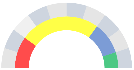
- For this, right-click on the chart and then click on “Select data”.
- In the “Select Data Source” window, click on “Add” to enter a new series under “Legend Entries” and select the “Values” column from the third data table.

- After that, select the chart and go to the Chart Design tab ➜ Change Chart Type (Chart Tools ➜ Design in older versions).

- In the “Change Chart Type” window, select Combo, choose Pie for the “Pointer” series, and click OK.
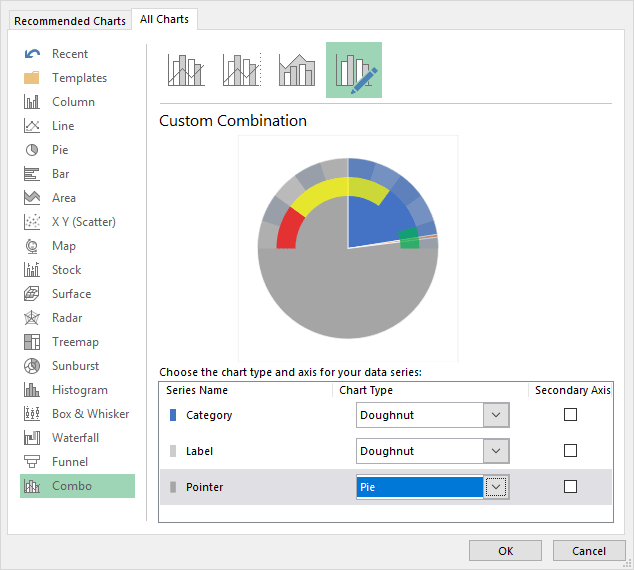
- At this point, you have a chart like below. Note: If, after selecting a pie chart, the angle is not correct (there is a chance), make sure to change it to 270°.

- Now, select both of the large data parts of the chart and apply no fill color to them to hide them.
- After this, you’ll only have the small part left in the pie chart which will be our needle for the SPEEDOMETER.
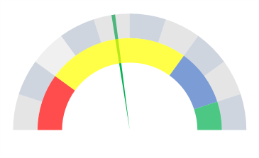
- Next, you need to make this needle bit out from the chart so that it can be identified easily.
- For this, select the needle and right click on it, and then click on “Format Data Point”.
- In “Format Data Point”, go to “Series Options” and add 5% in “Point Explosion”. At this point, you have a ready-to-use SPEEDOMETER (like below); just a final touch is required and that final thing is adding data labels and we need to do this one by one for all three charts.

- First of all, select the category chart and add data labels by Right-Click ➜ Add Data Labels ➜ Add Data Labels.
- Now, select the data labels and open “Format Data Label” and after that click on “Values from Cells”.
- From here, select the performance label from the first data table and then untick “Values”.
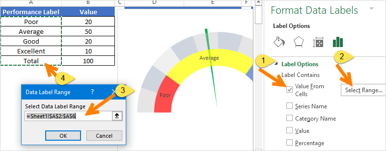
- After that, select the label chart and do the same with it by adding labels from the second data table.
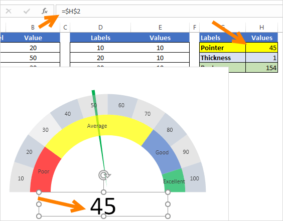
- And at last, you need to add a custom data label for the needle (That’s the most important part).
- For this, insert a text box and select it, and then in the formula bar enter “=” and select the pointer values cell, hitting ENTER.
- In the end, you need to move all data labels to end corners, like below:

Hurray! Your first Gauge/SPEEDOMETER chart is ready to rock.
How the Needle Data Works
The pie chart for the needle has three values: the pointer value, the size of the needle, and the rest of the circle. The total of all three must be twice the maximum of your scale, because only the top half of the chart is visible. So, with a scale of 0 to 100, the total is 200, and with a pointer of 68 and a needle size of 1, the third value is 131.
If the pointer value is in B1 and the needle size in B2, use the following formula for the third value, so the needle moves on its own when the pointer value changes:
=200-B1-B2
Change 200 to twice your own maximum if your scale is different. And keep the pointer value between 0 and the maximum, otherwise the needle goes into the hidden half of the chart. If the actual value is in A1, use the following formula for the pointer value:
=MIN(MAX(A1,0),100)
SPEEDOMETER – Why and Why Not
As I said it’s one of the most controversial charts. You can find a lot of people saying not to use a SPEEDOMETER or a GAUGE chart in your dashboards. I have listed some of the points which can help you decide when you can use this chart and when you need to avoid it.
1. Single Data Point Tracking
As we know, using a SPEEDOMETER can only be relevant (like Customer Satisfaction Rate) when you need to track a single data point. So, if you need to track data (like Sales, Production) where you have more than one point, then it’s not the right chart.
2. Only Current Period Data
This is another important point which you need to take care of while choosing a SPEEDOMETER for your dashboard or KPI reports: you can only present current data in it. For example, if you are using it to present the customer satisfaction rate, then you can only show the current rate.
3. Easy to Understand but Time-Consuming While Creating
As I said, a SPEEDOMETER is a single data point chart, so it’s pretty much focused and easy for the user to understand. But you need to spend a couple of minutes to create it, as it’s not there in Excel by default.
Conclusion
A SPEEDOMETER or a GAUGE chart is one of the most used charts in KPIs and dashboards. Even then you can find a lot of people who don’t like to use it at all.
But, it’s one of those charts (Advanced Excel Charts) which can help you make your dashboards look cool.
And that’s why I’ve not only shared the steps to create a SPEEDOMETER but also mentioned the points which you need to consider while using it in your dashboards. I hope you found it useful, but now, you need to tell me one thing.
Have you ever used a SPEEDOMETER or a GAUGE chart for your dashboard?
Share your views with me in the comment section; I’d love to hear from you, and please don’t forget to share this tip with your friends, I’m sure they will appreciate it.
Frequently Asked Questions
Why is my speedometer needle in the wrong place?
Check two things: the angle of the first slice must be 270° for all three charts, and the total of the needle values must be twice the maximum of your scale. If one of them is off, the needle points at the wrong value.
Can I use a speedometer for percentages?
Yes. Use 0 to 100 as the scale and enter the percentage as a number (68 for 68%), or use 0 to 1 with a total of 2 for the needle data.
What can I use instead of a speedometer chart?
For one value against a target, a bullet chart or a thermometer chart shows the same thing in less space, and both are easier to read in a dashboard.
Great post! I found the step-by-step instructions really helpful, especially the tips on customizing the gauge’s colors. I can’t wait to try this out for my project!