Let’s say you have a line-up of 20 products in your company and you have data for monthly sales of all 20 products.
From that data, you want to calculate the average of the top 5 products. In short, you want to get the average of the top 5 values from that data. Look at the below example.

Formula: Average TOP 5 Values
To average the top 5 scores from the list, you can use a formula based on the combination of LARGE and AVERAGE. And, the formula will be:
=AVERAGE(LARGE(B2:B21,{1,2,3,4,5}))
How this formula works
To understand this formula, you need to split it into two parts. In the first part, we used the LARGE function.
LARGE Function
The LARGE function can return the nth largest value from data. If you specify 2 as the nth value it will return the second-highest value from the data.
Here you need the top 5 values, not just one so that you will average them. For this, you need to enter the below array as the nth value.
{1,2,3,4,5}
When you enter this into the function, it returns an array of the top 5 values, just like the one below.
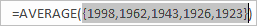
In the end, the average function returns the average of those values. Here you need to understand that the average function can take an array without entering a formula as CTRL + SHIFT + ENTER.
=AVERAGE(LARGE(B2:B21,{1,2,3,4,5}))
how to find product wise average value of largest 30 product.
We can not mention 1,2,…..30. How to combine 1 to 30 value in short like 1-30
Thanks….
https://prnt.sc/cnBDDdw7xcXJ
Thanks.
Thanks Puneet for Sharing.
However just I had a thought If I have a Large Data Set,It will not be possible to mention the array value uptill which I need to Calculate the Average.
We can instead use dynamic function like as I tried on my dataset:
“{=Average(If(Array of Rank DataRank,Array of Related Data))},Note – {}, Thsi will make it as Array Function by Cltr+Shift+Enter”.
Thanks!!
Anubhav
what is the difference if we use only =average(a1:a2) and =average(large(array,n))
What if your range is A1:A100? To find the average of the 5 largest values in a range using =average(a1:a5) requires the data in the range to be sorted largest to smallest (forcing them to be in the range A1:A5). Using the array formula =average(large(A1:A100,{1,2,3,4,5})) will choose the 5 largest values in the range no matter where they are in the range or what order they are in.
@plastic_cup:disqus More Power to You
10xx… i got it
You will get the average of the range, not just the top 5.