How to Sort in Excel – An Easy to Follow Guide

This is a complete guide to learning to sort data in Excel. In this tutorial, we will look at all the available options to sort the data. So, let’s get started.

Using the Sort Option

To open the sort order in Excel:

1. Go to the Data Tab.
2. In the Sort & Filter.
3. Click on the Sort Button.

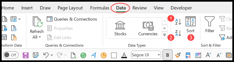
There are three buttons there which you can use to sort the data:

1. Smallest to Largest or A to Z – With this button, if you have numbers, you can sort data in smallest to largest order and if you have text, then you can sort it in A to Z order.
2. Largest to Smallest or A to Z – With this button, if you have numbers, you can sort data in the largest to smallest order, and if you have text, you can sort it in Z to A order.
3. Sort Button – You can open the “Sort” dialog box with this button.

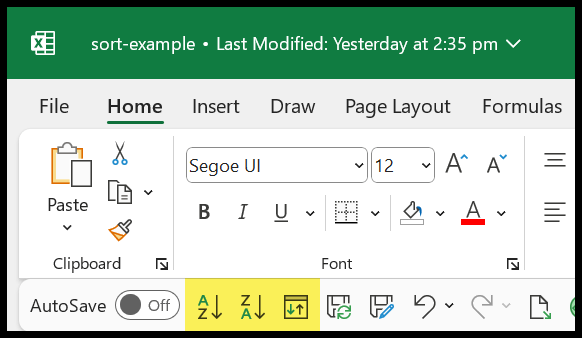
You can also add all these buttons to the quick access toolbar. With these buttons, you don’t need to go to the Data Tab when you want to sort data. These buttons are always available to use.

Open the Sorting Dialog Box

You can open the sorting dialog box from the Data tab or use the keyboard shortcut Alt > A > S > S.

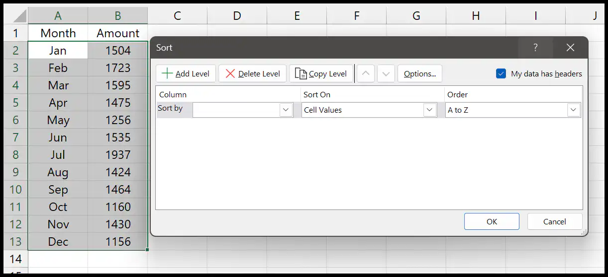
When you open the SORT dialog box, there are a lot of options that you can use. We will look at all these options later in this blog, but before that, we will try to sort the data.

Sorting Data in Excel

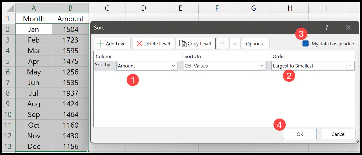
1. First, select the column name from the “Sort By” which you want to use for sorting. In this example, we are going to use Amount column which has numeric values.
2. After that, select the order from the “Order” and here we are using the “Largest to Smallest” as an order to sort the data.
3. Next, if your data has headers make sure to tick mark “My data has headers”. And if your data doesn’t have headers leave it unchecked.
4. In the end, click OK to sort the data.

Understanding All the Available Options in Sort Dialog Box

To use the SORT option in Excel effectively, you must know all the options available in the sort dialog box. So, let’s understand all the options one by one.

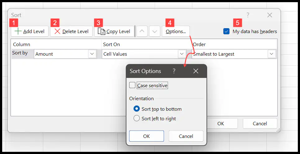
1. Add Level – Add more levels (columns) to the sorting with this button. That means you can use more columns (or rows) for sorting.
2. Delete Level – To delete a level. You can select a level and then click on the delete button to delete it.
3. Copy Level – With this, you can copy or duplicate a level you have already specified.
4. Options – This further has a few options which you can use. You can change the orientation of the sort. You can learn more about it from this quick tutorial which helps you to understand the horizontal sort.
5. My data has headers – This checkmark is checked by default. It tells Excel that the data you want to sort has headers. And if your data doesn’t have headers make sure to un-tick it.

Use a Custom List to Sort

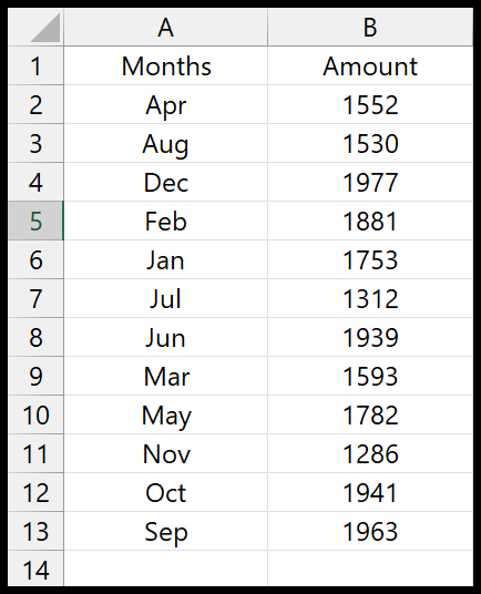
In the below example, we have a list of months with the amount. And in this data, the months are sorted alphabetically (A to Z). We have April month at the beginning and September at the end.

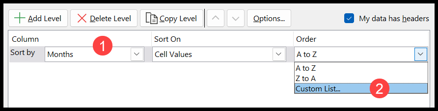
Now we will use the custom list order to sort months correctly. So, for this, open the sort dialog box and select the Months column from the “Sort By”. And after that, select “Custom List…” from the order.

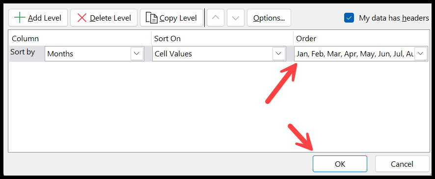
And the moment you select the “Custom List…” it opens a new dialog where you can select the list used to sort data. And here, we will use the list of short month names and click OK.

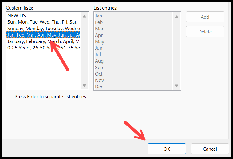
Now, you have the list of month names in the order to sort, and when you click OK, it sorts the data using the name of the months starting from Jan and ending in Dec.

Case Sensitive Sort

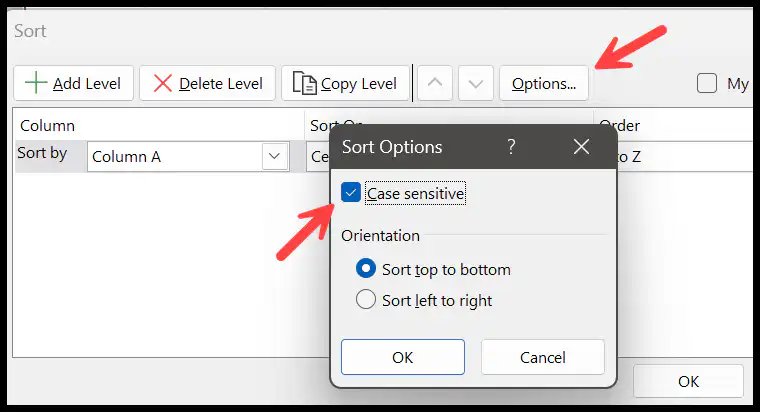
When you click on the “Options” button, you can select to apply the case-sensitive sorting. The case-sensitive sorting will put value with the first letter upper case first and then value with the first alphabet lower case.  

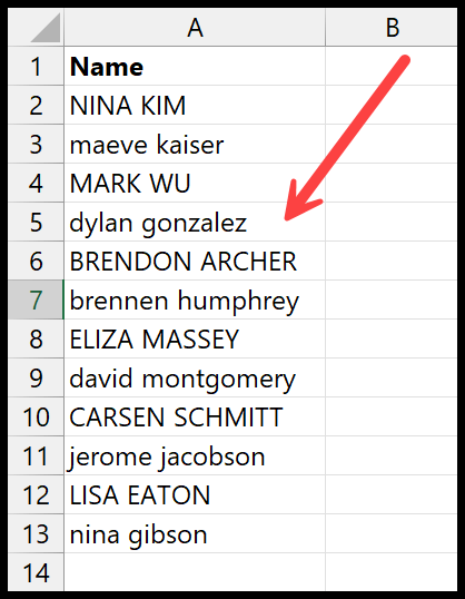
You can see in the example below; we have a list of names where some are in upper case and some are in lower case.

And when you tick mark the case-sensitive option while sorting the data, it sorts data by considering both upper and lower case values.

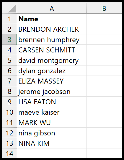
In the above example, both names start with B & b and the name with C after these.

Sort by Cell Color or Font Color

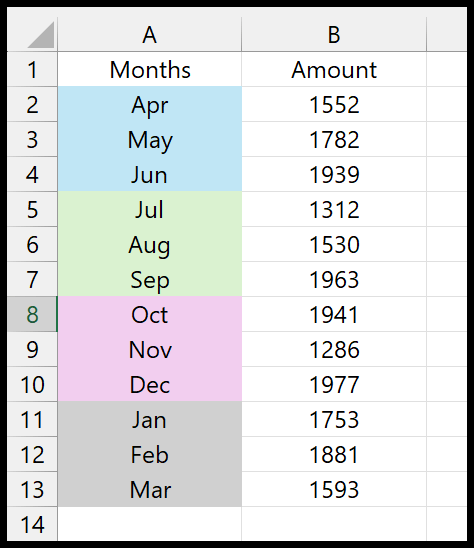
You can also sort data using the cell color or font color. In the example below, we have a color for each set of three months. Now we need to sort the data in a way that April-Jun should be at the top, and Jan-Mar should be at the bottom.

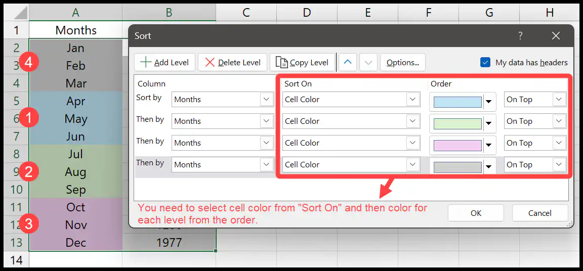
First, you need to create multiple levels to use this cell colour sort option. And in each level, you need to define the color you want to get on the top.

As you can see, the color we used in the first level in the Apr-Jun month. And then, Jul-Sep’s color, Oct-Dec’s color, and in the end, Jan-Mar’s color. And the moment you click OK, it sorts the data using the sort order we specified.

And in the same way, you can sort the data using the font color instead of the cell color. You only need to select the “Font Color” option from the “Sort On”.

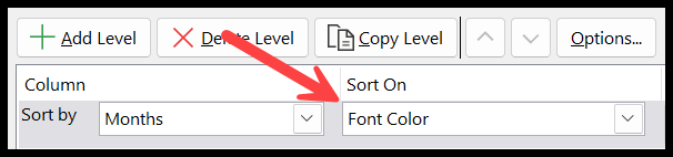
The rest of the steps are the same as we have used in the “Cell Color”.

Sort by Conditional Formatting

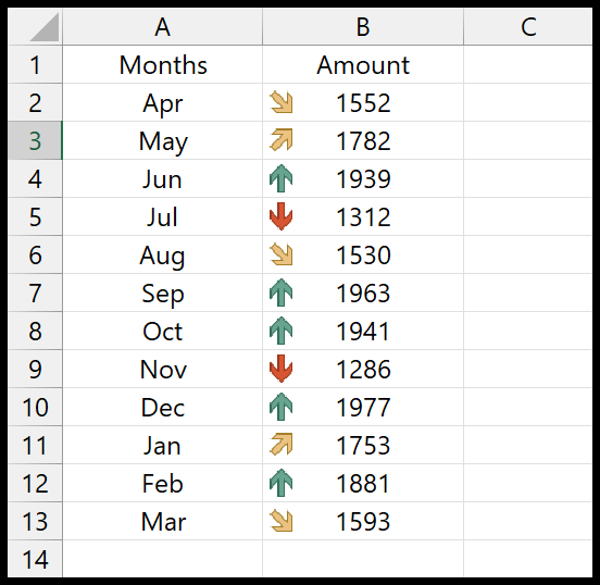
The sort dialog box also allows you to sort cells based on conditional formatting icons. In the example below, you can see four kinds of arrows on the amount column values.

Now, when you open the sort dialog box, add levels to sort data based on the icons.

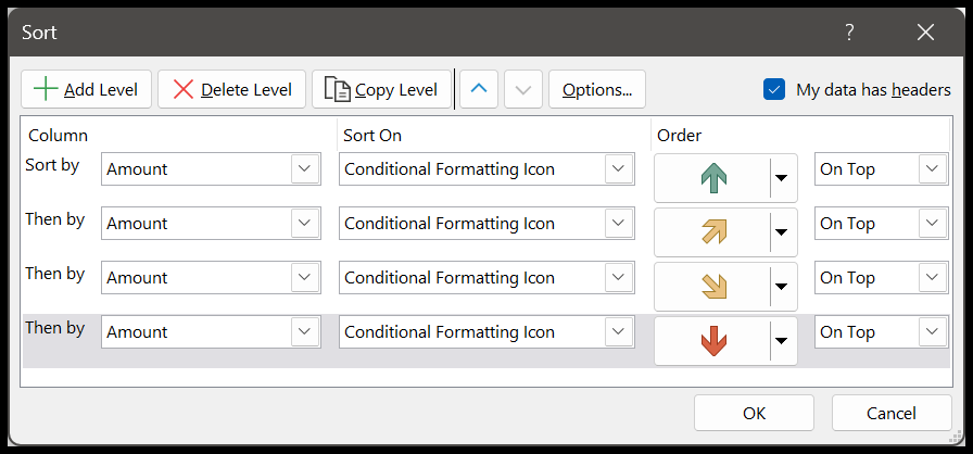
From the “Sort On” dialog box, select the “Conditional Formatting Icon” and select the icon you want to put on the top while sorting. In the above example, we have four levels of sorting to sort all four icons.

And when you click on OK to sort, it sorts data based on the levels you have specified.