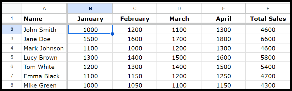
I have data to track your team’s performance using Google Sheets. I have a workbook where each row shows a different sales representative, and each column shows their monthly sales.
To keep things organized, you want to keep the names of the sales representatives always visible while I scroll through the data. It is where freezing a row or column can help.
When you freeze a row or a column, a grey line always indicates that it is frozen.
This tutorial will look at simple steps to freeze a row or column or freeze rows and columns starting from a specific cell.
Benefits of Freezing Rows and Columns
Freezing rows helps you keep important information, like headers, visible while you scroll through your data.
This makes understanding and comparing data easier because you always know what data each column has. You don’t need to go back to the top of the data and see the header to understand your data type in a column.
Freeze the First Row or Multiple Rows
In Google Sheets, you have the option by default to freeze the first row instantly.
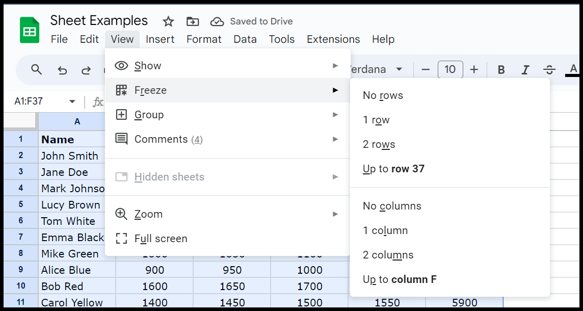
To freeze the first row in your worksheet, go to “View”, and then from there, go to the dropdown menu, choose “Freeze,” and then select “1 row.”
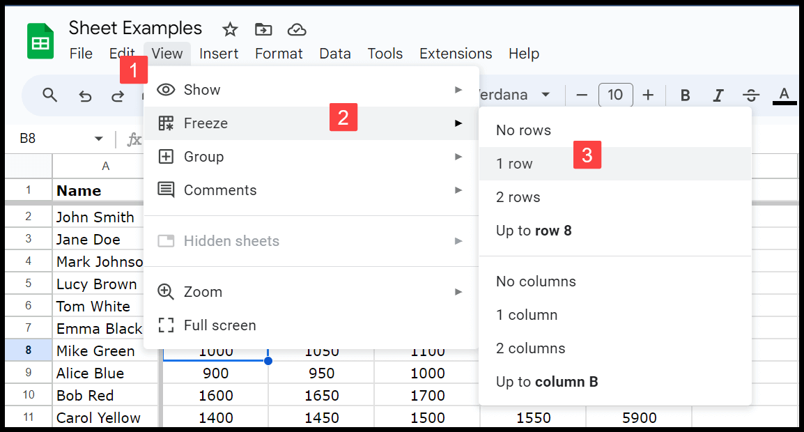
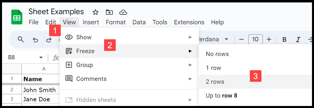
In the same way, you have the option to freeze the second row as well. Just below the “1 Row,” you have the option “2 Row,” when you click on it, it will freeze row 2.
The first two rows will freeze when you scroll down to the data in the worksheet.
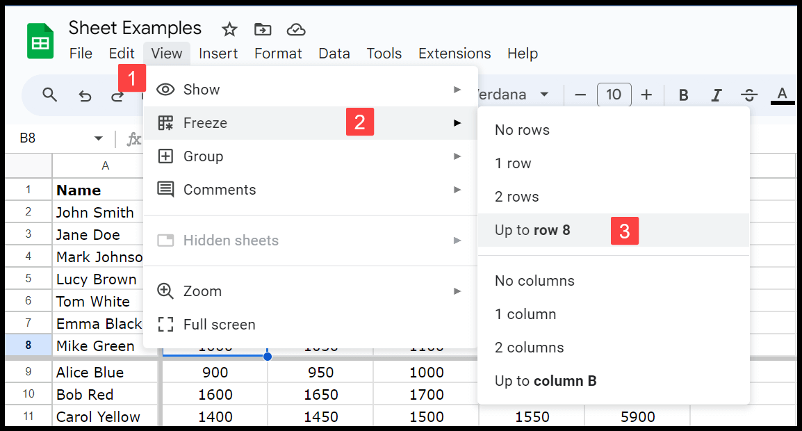
You can also freeze multiple rows from the same list of options. Let’s say you want to freeze starting from the 8th row. Select any cells from the 8th row and then go to View > Freeze > Up to row 8.
These frozen rows will stay there when you scroll through the data.
Note – If a worksheet is locked and you don’t have the right to edit that worksheet, you won’t be able to freeze a row or column from that worksheet.
Read Also – Group Rows in Google Sheets / Delete Rows in Google Sheets
Freeze the First Column or Multiple Columns
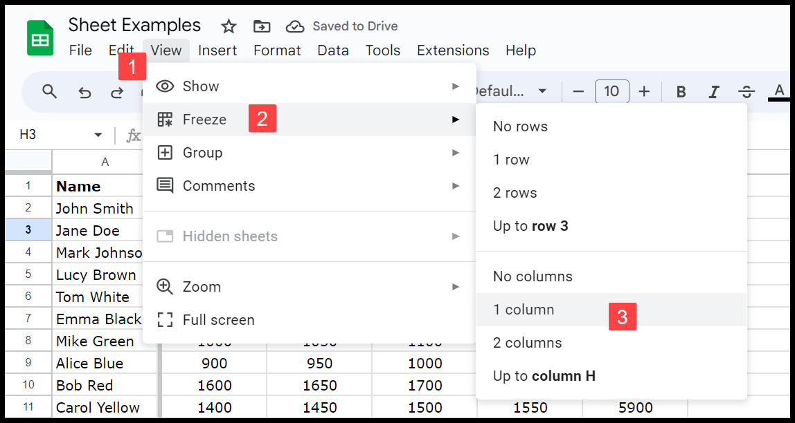
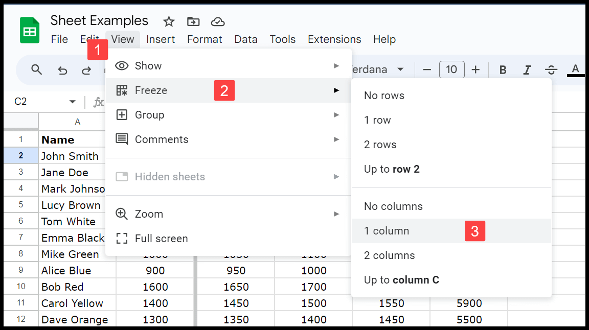
Like rows, you have a separate option to freeze columns. When you go to View > Freeze, you will see a list of options for freezing the columns. Let’s you want to freeze the first column; in this case, you can select the option you have there, “1 column”.
You also have an option to freeze the first two columns. In the list of options, you have the option “2 columns”, which freezes the first two columns. With this, the first columns will freeze when you move to the right of your worksheet.
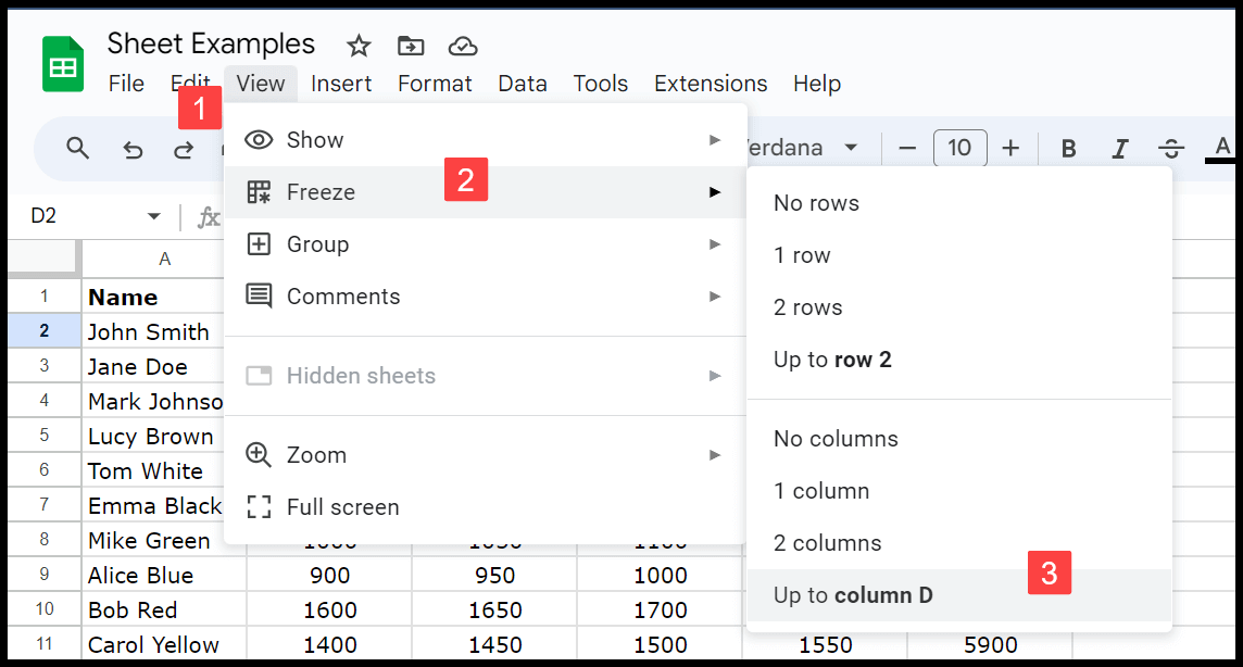
As we have learned about rows, you have the option to freeze multiple columns up to the column you want. Let’s say you want to freeze up to column D.
You can select a cell from column D and then click on the option “Up to column D.”
Freeze a Row or Column Starting from a Cell
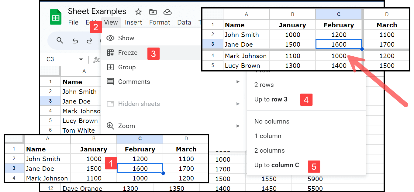
Let’s say you want to freeze rows and columns starting from cell C3. This means three rows and three columns need to be frozen. You must select cell C3 and then go to View > Freeze. From there, you need to activate two options: freeze the column and then the row.
Keyboard Shortcut to Freeze Row and Column
There is no direct keyboard shortcut to freeze a row or a column, but you can open the View menu with a keyboard shortcut and then use the keys further to apply the options.
Press Alt + Shift + V to open the “View” menu. Next, press R to select the “Freeze” option. To freeze rows, press 1 to freeze up to the current row. For columns, press C to freeze up to the current column.